What Meets the Eye

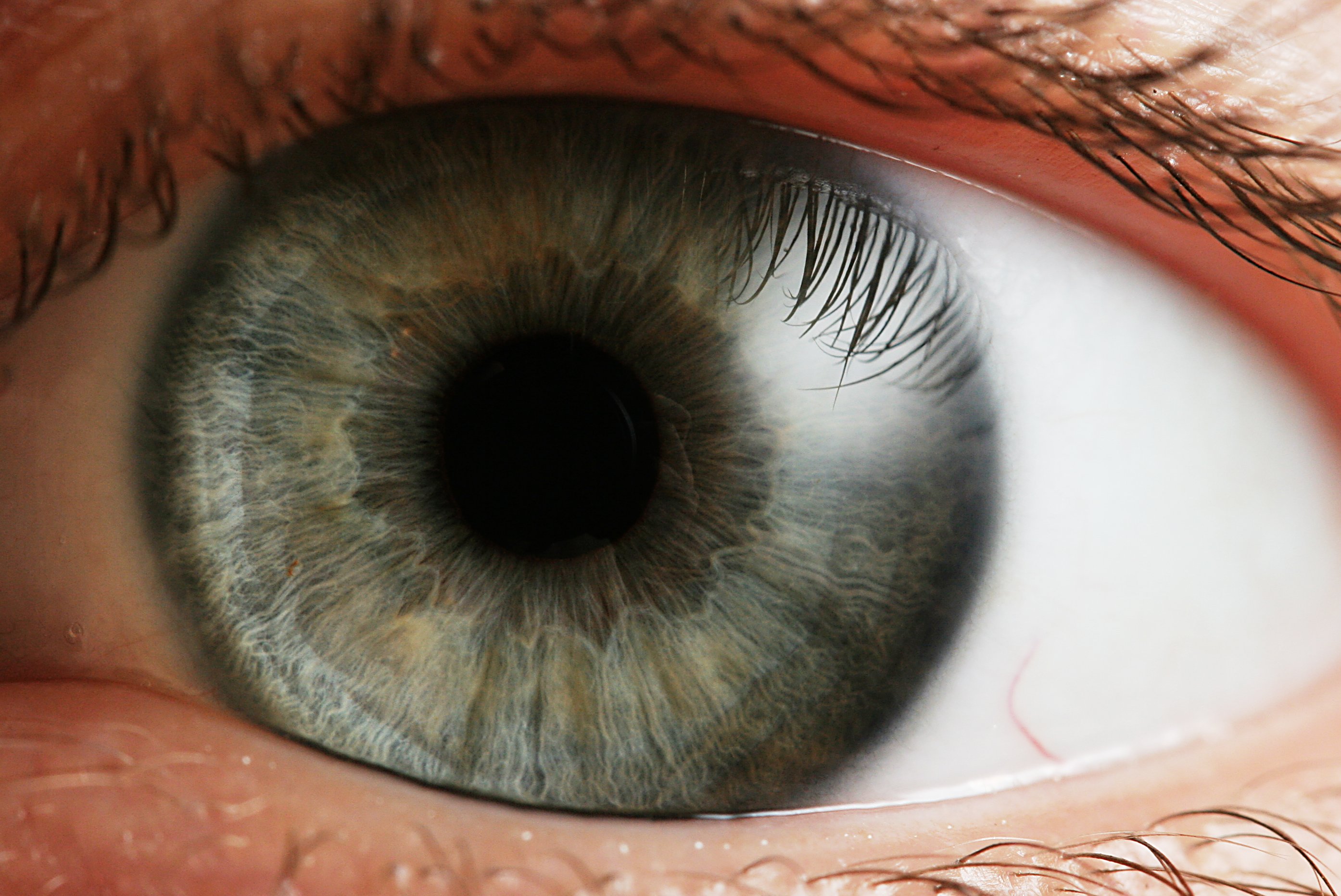
Some time ago, I read a report stating that about half of American adults—including many college students—understand basic science so poorly that they think that rays shoot out of their eyes.

This idea had already been widely dismissed as incorrect about 700 years ago (roughly ±300 years), and modern scientific understanding of light itself has not changed significantly in the last 100 years.

Though the report is now 20 years old, the level to which average Americans understand science—and in many cases basic facts—seems to decrease. For example, around the 50th anniversary of the first people landing on the Moon, one 2019 poll showed that only 82% of American adults under 35 believe that it actually happened, versus 97% of those at least 55 years old—old enough to have seen the event on live television. (There also exists significant third-party evidence for the Apollo Moon landings, including the presence of retroreflectors on the Moon—some left by crewed missions—that are regularly observed from Earth.)

A Very Brief Summary of How Vision Works

The light you see comes from somewhere—whether from as far away as our Sun (or other stars even further away), or from something nearby such as a camp fire, a light bulb, or even a matrix of tiny light-emitting diodes in the display of a smart phone in your hand. In each case, light is a bunch of subatomic particles called photons. Photons are generally created by heating things up, increasing the the energy stored in the atoms that each thing is made of and effectively boiling photons out of them, like steam released while heating water.

Photons travel as tiny waves, wiggling back-and-forth at constant rates that we call frequencies, which describe how frequently each wiggle reaches its peak in one particular direction before heading the other way. The different wavelengths of these wiggles are what our eyes interpret as colors. (The direction of the wiggle in relation to the photon’s direction of travel stays pretty constant, too; that’s called its polarization.) Each photon travels in a straight line through the center of its little wiggles until something causes it to change its course, such as reflecting off a surface or refracting through something like glass or droplets of water vapor in air, which is what causes us to see colors in the daytime such as blue skies, a red sunrise or sunset, and sometimes rainbows.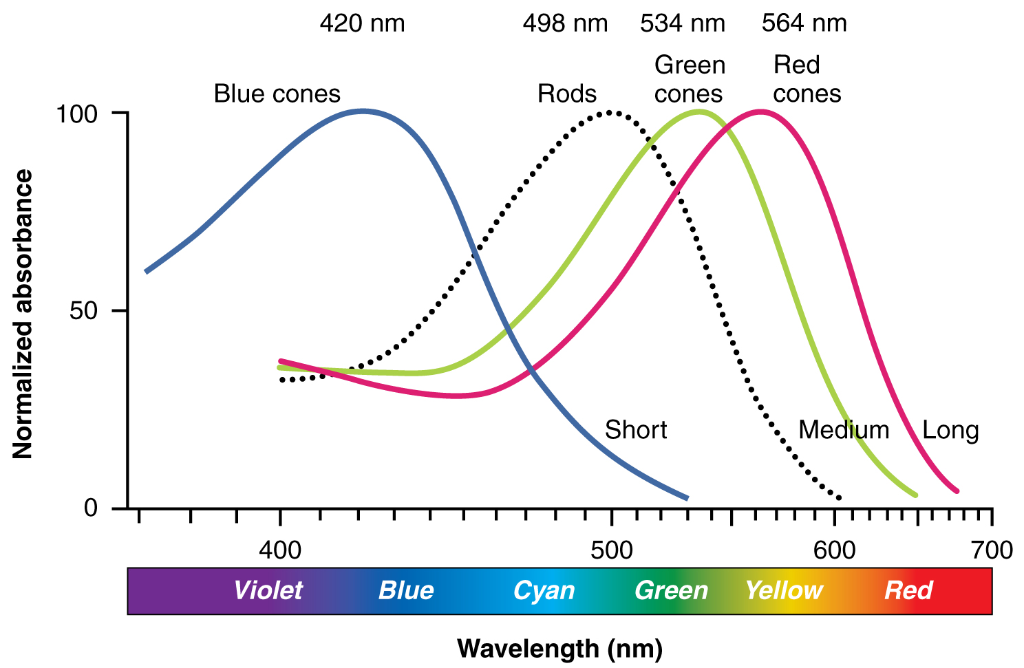

When they reach the area at the back of our eye (the retina), photons of different wavelengths fit in four different sizes of photoreceptor cells like fitting different coins only into certain slots of a machine. (Though I expect that the waves of photons with longer cyclic periods have greater amplitude so they all travel at the same rate, I’m not sure whether this has been determined.) These cells have two types named after their shapes: rod cells providing sensitive night vision and cone cells differentiating between three colors.

Illustrated to the right are the sensitivities of each of these types of cells to photons of different wavelengths. The wavelengths of peak sensitivity is indicated for each type. (Note that the colors to which cone cells are most sensitive are not perfectly red, green, and blue—as indicated—but instead are yellowish green, cyanish green, and blue, respectively.)

The energy from photons striking the atoms of those cells cause them to release electrons through a conversion process called the photoelectric effect (which again works a little like releasing steam from boiling water). The electrons then travel through your nerve cells as signals to your brain. This .

For discovering the photoelectric effect (and much more), the German-born theoretical physicist Albert Einstein (1879-1955) was awarded the 20th Nobel Prize in Physics (nominally for 1921), which he received in 1922.

Now being 100 years later, this seems like a good time to celebrate the achievement.

What Is Light?

The way our sense of vision works has been a mystery, and many people contributed to the story. Like any good mystery, it has taken much time and effort to unravel, and there’s always more than meets the eye.

Through a span of more than 2000 years, many theories about visual perception, light, and color have been proposed, refuted, confirmed, and refined—evolving as science does.

But one thing is clear: vision depends on light.

There are many ways to describe light; I include a few below.

Light Travels in Rays to Our Eyes, Not From Them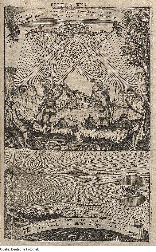

The Sicilian Greek pre-Socratic philosopher Empedocles (c. 494 - c. 434 BCE)—best known for originating the cosmogonic theory of the four classical elements of water, earth, fire, air—attempted to explain vision with an emission theory (or extramission theory), through which fiery rays come from the eyes (eye beams) and interact with fiery rays from a source such as the Sun.

This idea was held by prominent scholars spanning centuries, including:

• the Athenian Greek philosopher Plato (c. 426 BCE - c. 348 BCE) around 400 BCE,
• Euclid who wrote around 300 BCE in his books Optics (Optica) about direct vision and Catoptics about vision by reflection,
• the Roman mathematician, astronomer, astrologer, geographer, and music theorist Ptolemy (Claudius Ptolemy, c. 100 - c. 170) who in his book Optics developed prior ideas and described refraction, and
• the Greek Roman physician, surgeon, and philosopher Galen (Aelius Galenus, Claudius Galenus, or Galen of Pergamon, 129 - c. 216).

The direction the rays traveled was corrected—as light to the eye—by the Muslim Arab mathematician, astronomer, and physicist Ḥasan Ibn al-Haytham (Latinized as Alhazen or Alhacen, c. 965 - c. 1040) through his seven-volume treatise Book of Optics, published in Arabic 1011 to 1021, and translated into Latin by an unknown scholar around the end of the 12th century.

In 1490, the Italian painter, draughtsman, engineer, scientist, theorist, sculptor, and architect Leonardo da Vinci (1452-1519) included extramissionist statements his notebooks (Ackerman 1978, qtd. in 2002 by Winer et al) so it seems likely that these beliefs continued to be held at least in some scientific circles until after Alhazen’s work was printed in 1572 by Friedrich Risner (c. 1533-1580) as part of his collection Opticae thesaurus: Alhazeni Arabis libri septem, nuncprimum editi; Eiusdem liber De Crepusculis et nubium ascensionibus, Item Vitellonis Thuringopoloni libri X (“Optical Treasure: Seven books of Alhazenus the Arab, published for the first time; His book On the Crepuscles and Ascensions of the Clouds, Also of Vitello Thuringopol”).

This view may have persisted until the German astronomer, mathematician, astrologer, and natural philosopher Johannes Kepler (1571-1630) paused his other work to focus on optical theory for most of 1603, and on 1 January 1604 presented his emperor with the resulting manuscript, which was published as Astronomiae Pars Optica (“The Optical Part of Astronomy”).

Light is Rays from Afar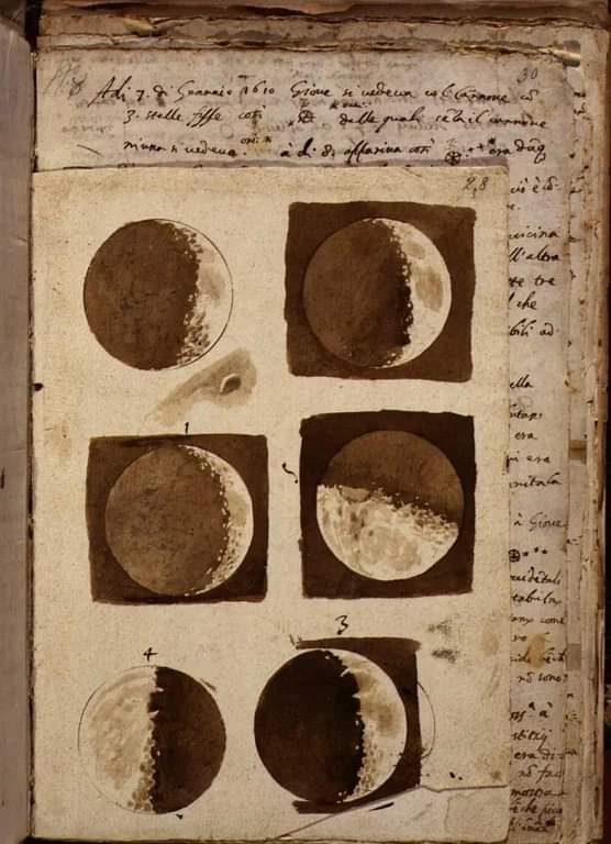

The first record of a telescope was a 1608 Dutch patent; Galileo Galilei (1564-1642) had constructed one and with it sketched the Moon the following year, in 1609. (See image at right.)

Only 360 years later, in 1969, the first footprints were placed on the Moon—an event viewed by millions of people on Earth via live television, including the inventor of electronic television Philo Farnsworth (1906-1971); in 1996 his widow Elma “Pem” Farnsworth said of the event, “We were watching it, and, when Neil Armstrong landed on the moon, Phil turned to me and said, ‘Pem, this has made it all worthwhile.’ Before then, he wasn’t too sure.”

Light is a Spectrum of Colors (Visible to Most)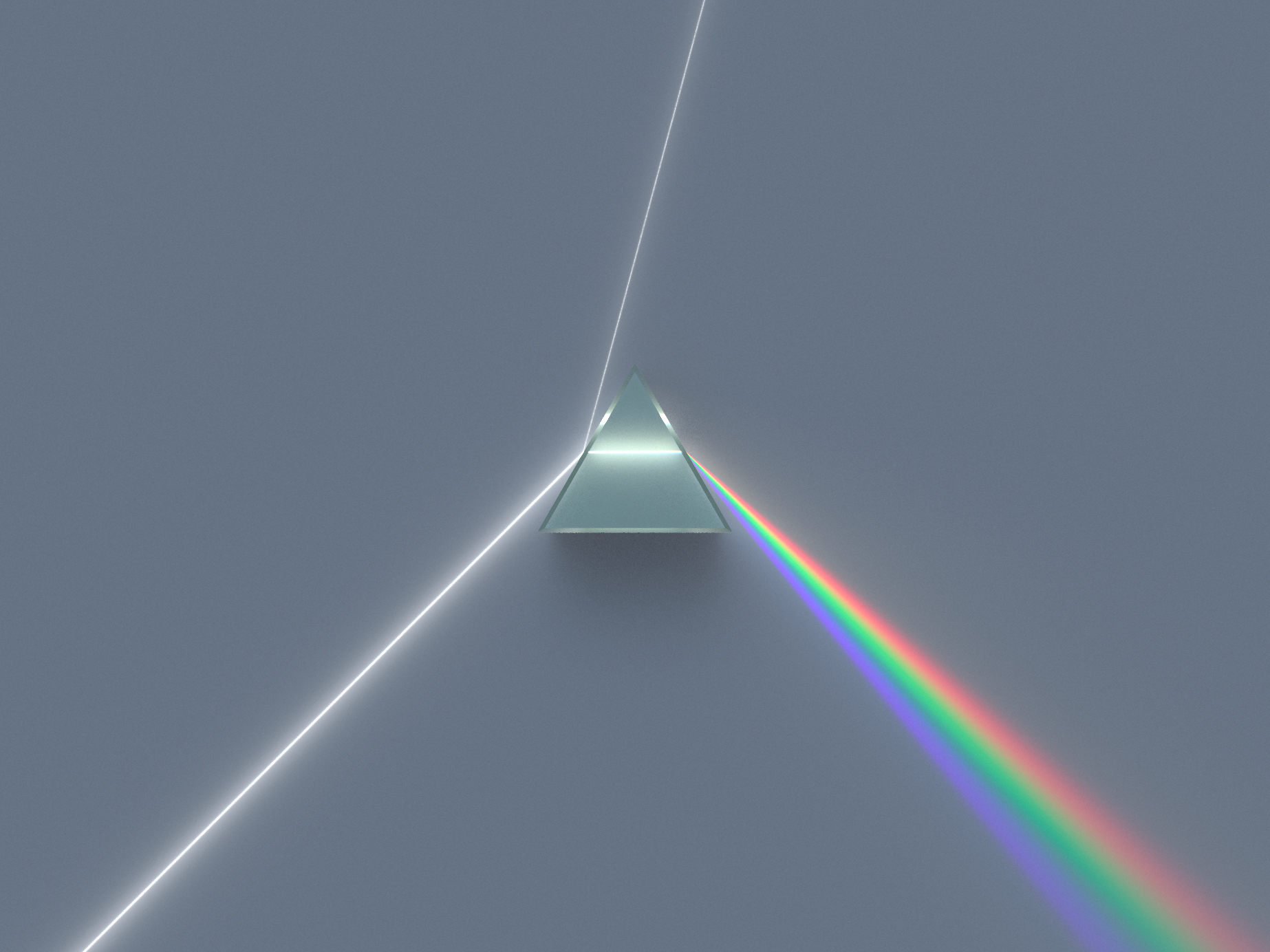

Early telescope lenses shared a defect called chromatic aberration, which caused the locations of features of different colors to appear distorted relative to each other.

Apparently prompted by this, the English mathematician, physicist, astronomer, theologian, and author Isaac Newton (1643-1727) in 1666 started using a prism to dissect visible light into its component colors; to describe them and their order he borrowed the word spectrum, which had entered the English language in the 1610s to describe apparitions and specters. That white light was composed of light of different colors was one of several ideas Newton published in his 1704 book Opticks.

(About 269 years later, such a demonstration also inspired the cover of the 1973 music album Dark Side of the Moon by Pink Floyd, which looked something like the illustration at right.)

The problem of chromatic aberration was solved in 1733 with the invention of the achromatic lens. In 1668, Newton provided an earlier (and in many ways simpler) solution by creating the first practical reflecting telescope—a type still used today, including by the Hubble Space Telescope (HST, launched 24 April 1990) and James Webb Space Telescope (JWST, launched 25 December 2021).

In 1798, the English chemist, physicist, and meteorologist John Dalton (1766-1844) published the first scientific paper on color blindness, Extraordinary Facts Relating to the Vision of Colours, after realizing his own color blindness. The most common type is red-green color blindness (Dalton’s), which affects about 8% of males vs. only 0.5% of females (at least among people of northern European descent).

Light is Part of a Broader Spectrum

Since Newton’s discovery of the component colors of visible light, the spectrum was expanded to include invisible light. In 1800, the astronomer William Herschel (1738-1822) discovered what we today call infrared light. In 1801, the German physicist Johann Wilhelm Ritter (1776-1810) discovered ultraviolet light.

In 1845, by English physicist and chemist Michael Faraday (1791-1876) first linked light to electromagnetism and thus expanded our understanding of light to create the modern electromagnetic spectrum. In the 1860s the relationship was described by James Clerk Maxwell through four partial differential equations for the electromagnetic field (Maxwell’s equations).

This spectrum was again expanded in 1866, 1895, and 1900 when—respectively—the physicist Heinrich Hertz generated and detected what we now call radio waves, Wilhelm Röntgen (1845-1923) discovered what he called X-rays (in 1901 earning him the first Nobel Prize in Physics), and Paul Villard discovered gamma rays.

Light is the Fastest Thing (When Not Impeded)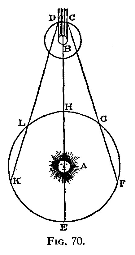

Since at least as early as the ancient Greeks, whether light traveled instantaneously or at a very fast finite speed had been debated.

The first quantitative estimate of the speed of light is usually attributed to the Danish astronomer Ole Rømer (Olaf Rømer, 1644–1710), who while working at the Royal Observatory in Paris in 1676 timed eclipses of Io, the innermost of Jupiter’s four Galilean moons (and one of 80 moons now known to orbit Jupiter). The Dutch mathematician, physicist, astronomer, and inventor Christiaan Huygens (also spelled Huyghens, 1629-1695) combined this with an estimate for the diameter of the Earth’s orbit to estimate the speed of light to be 220,000,000 meters per second (m/s).

This first estimate was about 26% lower than the speed of light we know today.

In 1905, Albert Einstein published four papers, which are now described as his Annus Mirabilis papers (“miracle year” papers). The third paper presented his special theory of relativity (often shortened to special relativity and sometimes abbreviated SR), which establishes the prohibition of motion faster than light—effectively establishing the speed of light through a vacuum as the speed limit for all matter and energy.

Since 1983, the speed of light through a vacuum has been defined as 299,792,458 m/s. This is often represented using the universal constant c.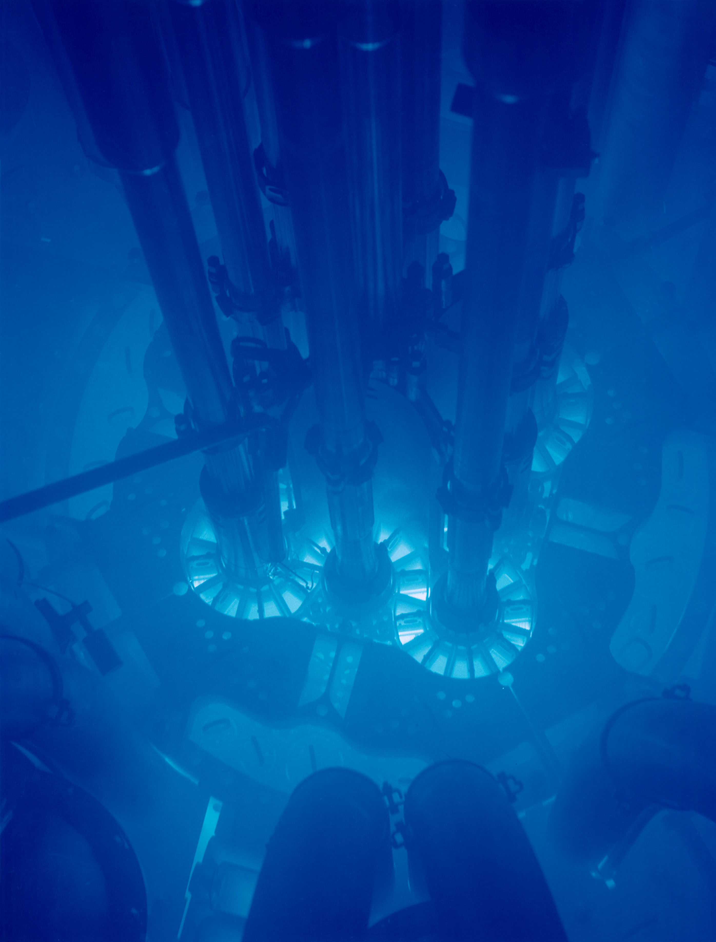

In 1637, the French philosopher, mathematician, and scientist René Descartes (1596–1650) published a theory of the refraction of light that assumed that light—like sound waves—would travel faster in a denser medium than in a less dense medium; today we know that the opposite is true. Through air, light travels slower than its speed in a vacuum—but only by about 0.03%, which is small enough that it may often be dismissed as negligible. Through water, light travels 25% slower, which allows radioactive decay to cause an interesting glow through an optical analog to a sonic boom called Cherenkov radiation—named after the Soviet physicist Pavel Cherenkov (1904-1990), who shared the 52nd Nobel Prize in Physics in 1958. In 2001, it was demonstrated that light could be slowed even to a stop.

In 2011, an anomalous report from the OPERA experiment suggested that faster-than-light speed had been measured in muon neutrinos. (The existence of the muon neutrino was proved in 1962 by Leon M. Lederman, Melvin Schwartz, and Jack Steinberger, who together shared the 82nd Nobel Prize in Physics in 1988. The first neutrinos had been detected in 1956 by Frederick Reines, who shared with Martin Lewis Perl the 89th Nobel Prize in Physics in 1995; the electron neutrino was the first type discovered, and is now one of three in the Standard Model of particle physics. These are types of leptons, which—along with quarks—are the two types of elementary fermions, which are one of two classes of elementary particle—the other class being elementary bosons.) By 2012, the speed of these neutrinos had been found to be consistent with the speed of light.

Light is a Particle and a Wave

In 55 BCE, the Roman poet and philosopher Lucretius (Titus Lucretius Carus, c. 99 - c. 55 BCE) wrote in On the Nature of the Universe that light is “composed of minute atoms,” an idea validated and refined starting in 1905 by Albert Einstein when he theorized that light consists of a type of quantum subatomic elementary particle, which we recognize today as a type of boson called a photon.

These subatomic particles were named, respectively, in 1924 by Paul Dirac (1902-1984, 1933 co-recipient of the 31st Nobel Prize in Physics) for the contributions of Satyendra Nath Bose (1894-1974) and in 1926 by Gilbert N. Lewis (1875-1946); the names follow (and reinforce) the convention of suffixing “-on” (from the ancient Greek ending “-ον” on neuter nouns and adjectives) since 1894 when the Irish physicist George Johnstone Stoney (1826-1911) suggested replacing the term he coined in 1881 (“electrolion”) with “electron,” which is a portmanteau combining parts of the words “electric” and “ion.” The words “electric” and “electricity” are derived from the Latin “ēlectrum” (also the root of the alloy electrum), which came from the Greek word for amber (fossilized tree resin), ἤλεκτρον (ēlektron); the ancient Greeks had noticed that amber attracted small objects when rubbed with fur, an effect of what we recognize today as static electricity. The word “ion” was introduced in 1834 by English physicist and chemist Michael Faraday (1791-1876) after a suggestion by the English scientist, Anglican priest, philosopher, theologian, and historian of science William Whewell (1794-1866).

Photons along with gluons and W and Z bosons are the four force-carrying fundamental particles (called gauge bosons) in the Standard Model of particle physics, which evolved from 1954 and was named in 1973 by Steven Weinberg (1933-2021) who—with Abdus Salam (1926-1996) and Sheldon Lee Glashow (born 1932)—in 1979 shared the 73rd Nobel Prize in Physics. The use of the term was extended with experimental confirmation of the existence of four quarks (including electroweak theory in 1975), the tau neutrino (in 2000), and the Higgs boson (in 2012).

A photon behaves with duality: both as a massless particle and as a wave.

As a wave, the frequency at which a photon oscillates depends upon the speed at which the photon travels and the oscillation’s wavelength. This relationship is conventionally described by the equation

ν = c ÷ λ

in which:

ν (nu)

is the photon’s frequency in hertz (Hz) & often on the order of terahertz (1 THz = 10¹² Hz),

λ (lambda)

is the photon’s wavelength in meters (m) & often on the order of nanometers (1 nm = 10^-9 m), and

c

is the speed of light (the photon’s speed), which (as described earlier) in a vacuum is 299,792,458 m/s.

I believe (though I’m unable to find much literature on the subject) that the waveform of a photon is sinusoidal—like a sine wave, with a smooth periodic oscillation in a plane (the direction of its polarization) about an axis defined by the photon’s overall direction.

The following table includes many names given to photons based on their frequencies, in decending order (from highest to lowest). Note that some boundaries may be approximate or overlap due to differing definitions.

Types of Electromagnetic Energy

Frequency	Description of Photons
	Gamma Rays (γ)
30 EHz (1018)
	X-Rays (incl. X-ray background)
30 PHz (1015)
		Extreme Ultraviolet (EUV) Light	Vacuum Ultraviolet (VUV or G) Light
3 PHz (1015)
2.5 PHz (1015)	Ultraviolet C (UV-C) Light
		Far Ultraviolet (FUV) Light
1.5 PHz (1015)
1.1 PHz (1015)		Middle Ultraviolet (MUV) Light	Ultraviolet Light
1 PHz (1015)	Ultraviolet B (UV-B) Light
950 THz (1012)		Near Ultraviolet (NUV) Light
	Ultraviolet A (UV-A) Light
790 THz (1012)
750 THz (1012)			Visible Light (incl. Extragalactic Background Light)
430 THz (1012)
400 THz (1012)	Infrared A (IR-A) Light
		Near Infrared (NIR) Light	Infrared (IR) Light (incl. Cosmic Infrared Background)
215 THz (1012)
	Infrared B (IR-B) Light	Short-Wavelength Infrared (SWIR) Light
100 THz (1012)
	Infrared C (IR-C) Light	Mid-Wavelength Infrared (MWIR) or Intermediate Infrared (IIR) Light
37 THz (1012)
		Long-Wavelength Infrared (LWIR) Light
20 THz (1012)
3 THz (1012)		Far Infrared (FIR) Light
300 GHz (109)			Radio Waves
	Microwaves (incl. Cosmic Microwave Background)
300 MHz (106)
3 Hz (100)
	Thermal Radiation

Light is a Form of Radiation

Light is emitted from most sources in all directions.

To describe such motion outward from a center, the terms “radiation” and “radioactivity” (from the Latin radius, meaning “ray”) were introduced by the Polish-born French scientist Marie Curie (1867-1934, born Maria Salomea Skłodowska, also known as Madame Curie) and by 1898 replaced the term “Becquerel rays” for describing atomic nuclear decay as “spontaneous radioactivity,” which was discovered in 1896 by French physicist and engineer Henri Becquerel (1852-1908). For this, he, she, and her husband and fellow scientist Pierre Curie (1859-1906, whom she met in 1894 and married in 1895) were awarded the third Nobel Prize in Physics in 1903.

(Marie Curie was also the first woman to receive a Nobel Prize. For discovering the atomic elements radium and polonium, in 1911 she was also awarded the 11th Nobel Prize in Chemistry, making her the first person and the only woman to be awarded two, and the only person to do so in two scientific fields; she and her husband became the first married recipients and launched the Curie family legacy of four prizes and five individual laureates. In 1906, she became the first female professor at the University of Paris. In 1911, the French Academy of Sciences narrowly failed to elect her as a member; due in part to sexism in academia, it did not include a female member until 1962 when it elected a doctoral student of Curie’s, Marguerite Perey, who lived 1909-1975.)

To simplify understanding and calculations, radiation (such as light or other electromagnetic energy) is often described as coming from a point source.

Energy that is radiated outward evenly in all directions decreases in density proportionally with distance from its source; we can visualize and calculate this as dividing an amount of energy over the area of a sphere as its radius increases using an inverse-square law. For example, the amount of light from a bulb or the sun that reaches one surface will be only one-fourth as much as that reaching a surface only half as far away from the source.

Some forms of radiation are necessary to life, such as heat and as sunlight. Yet, radiation at high energies and/or in large amounts cause illness, lower life expectancy, and—in extreme cases—can kill immediately.

This harmful high-energy radiation includes ionizing radiation such as particle radiation (alpha radiation, beta radiation, and neutron radiation) and also radiation of electromagnetic energy at frequencies higher than roughly 2.4-7.25 petahertz (PHz, or 10¹⁵ cycles per second). High exposures can cause radiation burns and long-term or repeated exposure to elevated levels increase risks of radiation-induced cancers (radiation carcinogenesis). Electromagnetic energy at frequencies of about 1 PHz and higher (the upper spectrum from middle ultraviolet light and higher) also damages DNA though pyrimidine dimerization, causing sunburns and melanomas (skin cancers).

Even at lower frequencies, overexposure to large amounts of non-ionizing radiation causes burns. For example, in microwave ovens and near high-power radio transmitters, electromagnetic energy can heat and cook food or even living tissue.

Risks to eyes, sight, and vision include cataracts, which may be caused by enough electromagnetic energy at any frequency. Temporary or permanent blindness can be caused when an eye is exposed to bright light, such as a laser beam (see laser safety) or staring into a bright light source such as the Sun.

Radiation Safety, Atmospheric Absorbtion, and Altitude

My father was born in 1936 in Portland, Oregon. He grew up about 120 km (75 miles) down the Columbia River (northwest of Portland) in a rural community on Puget Island, which had been part of Oregon until the shipping channel (which defined the state line) had been moved to the south side of the island to facilitate the construction of a bridge that opened in 1939.

Along the river about half-way from Portland had been a facility Trojan Powder Works, where it manufactured gunpowder and dynamite (invented and patented in 1867 by the Swedish chemist Alfred Nobel, 1833-1896, who posthumously established the Nobel Prizes). (While still a boy, my father had relatively easy access to dynamite, but that’s another story.) Starting in 1970 (the year I was born), the site was used to construct the world’s largest pressurized water reactor (PWR).

Although the Trojan Nuclear Power Plant began commercial operation in 1976 and was licensed to operate for 35 years (to 2011), it was plagued by problems including major construction errors and a previously-unknown earthquake fault that were discovered during a routine shutdown in 1978, cracking steam tubes causing a shutdown for repairs in 1979, trouble restarting after a shutdown in 1984, and trace amounts of radioactive gases being released into the atmosphere in 1992, only a week after its owner successfully defeated two ballot measures (setting statewide campaign spending records) that would have closed the plant immediately. After documents citing safety concerns were leaked later that year, the plant was closed and dismantled. (Its cooling tower was later demolished using dynamite in 2006.)

Concerned by health risks to his side of our family living downstream from this leaky nuclear power plant, my father bought a simple and inexpensive electronic radiation detector with a loudspeaker—essentially a Geiger counter without the counter—hand-made by a local scientist from the former Soviet Union (which existed 1922-1991).

At one point after I had moved from California to Texas in 1993, I had borrowed the device and traveled via airline back to where I lived at the time. Mostly out of curiosity, I had briefly turned it on mid flight and recall it ticking somewhat more vigorously than usual, indicating higher exposure to radiation, as I might have expected at the higher altitude.

A flight attendent noticed and struck up a conversation about elevated rates of cancers among those within her industry. As I recall, she was concerned that it was about 10 times that of the general population. The little data I’ve seen since then suggests it might be closer to three times higher, which still seems significant.

Earth’s atmospere protects us by absorbing extraterrestrial radiation (both solar and cosmic). Earth’s gravitation causes the atmospere to be thicker at lower altitudes, and this additional thickness provides more protection. (The thickness of Earth’s atmosphere decreases as the square of the increase in altitude—like the inverse-square relationship described earlier.)

But airlines gain efficiency by flying their aircraft as high as they practically can—where the atmosphere is thinner and provides less resistance to the craft flying through it—and their cruising altitudes have been increasing. Though jet airliners had already entered service in 1958 (first used by Pan Am), The Twilight Zone’s 1963 episode Nightmare at 20,000 Feet suggests what common cruising altitudes were then (in addition to showing us William Shatner as a very nervous airline passenger before his role as a starship captain in Star Trek); as part of a 1983 feature film, the story was recreated as Nightmare at 30,000 Feet (starring John Lithgow in place of Shatner; Lithgow and Shatner comically alluded to these roles in their shared two-part episode of 3rd Rock from the Sun, ending its fourth season and airing May 25, 1999). Today, passenger airliners often cruise at altitudes of around 40,000 feet (flight level 400, abbreviated FL400, or nearly 12.2 km).

Even prior to its 1976 introduction, designers of the high-altitude supersonic Concorde jet airliners were concerned by potential exposure to harmful radiation from extraterrestrial sources such as cosmic radiation and unusual solar activity.

In 1994, the United States Federal Aviation Administration (FAA) recommended limiting average annual occupational exposure to 20 mSv. According to a 2003 report by the FAA, Americans each year receive on average about 2.95 millisieverts (mSv) of radiation from natural sources, including 0.27 mSv (9%) from galactic cosmic radiation. The United States Centers for Disease Control reports that current average annual exposure to cosmic radiation of 0.33 mSv being 11% of total natural radiation received, which I calculate would be 2.45 mSv, suggesting a 17% decrease in total natural radiation exposure. (I presume this variation might correlate and/or be caused by solar cycle, which repeats each 22 years—the Babcock Model—and nearly repeats each 11 years.) The FAA’s 1994 recommendation limits total radiation exposure to about 6.8 times this average level and implies limiting cosmic radiation exposure to 17.32 mSv, which is 64 times the average level.

Note also similar risks to astronauts.

Light is Transformed Through Absorbtion

The term absorbtion can be misleading, because energy absorbed by matter doesn’t disappear into it; it is transformed. In the case of visible light, what is not reflected as visible light is usually dissipated as heat; the energy entering and leaving the object are both photons, though the latter have much lower frequencies.

In theory, an object that would absorb energy ideally is called a black body, an idea introduced in 1860 by Gustav Kirchhoff (1824-1887); conversely, a body that reflects light instead of absorbing it would be a white body.

Real objects do not behave like either a theoretical ideal black body nor a theoretical ideal white body, but somewhere between the two. Real objects with conventional black paint will absorb about 97.5% of light; this has been increased to between about 99.6% and 99.9% (depending on the light’s angle of incidence) using super black and 99.965% using Vantablack, which entered production in 2014 and gets its name from VANTA, the acronym for vertically aligned nanotube arrays. Conversely, the most reflective surfaces—mirrors—vary in reflectivity based on their materials and configuration (e.g. first-surface mirrors versus second-surface mirrors using substrates such as glass or acrylic plastic), including (for most visible light) 25% for chrome, 85% for aluminum, 98-99% for silver, 99.9% for enhanced silver, and 80-99.999% or more for dielectric mirrors.

The temperature of an object describes the average level of excitation (energy) in the atoms from which the object is made.

According to the first law of thermodynamics (a version of the law of conservation of energy), the amount of energy in an object must be in equilibrium with the temperature of its environment, otherwise energy must be absorbed or dissipated as black-body radiation, a form of thermal radiation.

Light is Heat Energy

We can often sense that something is hot before we touch it. When we do, what we feel is mostly warm air around the object. It might contain some water vapor and maybe even visible steam.

But a warm object also emits photons, though usually they have such low energy that we can’t see them (though some of it was can detect with infrared cameras). Photons are carriers of heat; conversely, heat is photon energy.

Even in prehistoric times (before about 6000 BCE), people had already learned to heat things until they glowed red hot. (They even smelted metals.)

Nearly all solids and liquids will begin to glow as they are heated by their environments.

This process of taking in electromagnetic energy as longer-wavelength thermal radiation (heat), increasing the object’s temperature, and putting out electromagnetic energy as shorter-wavelength visible light (glowing) is called incandescence.

Most objects glow at the Draper point, which is 977°F (525°C, 798 K) and was established in 1847 by the English-born American scientist, philosopher, physician, chemist, historian, and photographer John William Draper (1811-1882).

For example, the colors of hot steel were given names at certain specific temperatures (by Stirling Consolidated Boiler Company in 1905, coincidentally Albert Einstein’s “miracle year”) and temperature ranges (in W. A. J. Chapman’s 1972 Workshop Technology, Part 1, 5th ed.), as noted in the table below. (Color samples are included where they appear on the selected source chart. A description of hexadecimal 24-bit color values is included in a following section.)

Colors of Hot Steel

Temperature*			Color	24-Bit Value	Name
Fahrenheit	Celsius	Kelvin			Stirling (1905)	Chapman (1972)
2730°F	1500°C	1773 K			white dazzling	white
2550°F	1400°C	1673 K			white bright
2397°F	1315°C	1588 K
2370°F	1300°C	1573 K		#FFE6AD	white heat	yellow white
2297°F	1259°C	1532 K
2190°F	1200°C	1473 K		#FFCF61	clear orange	yellow
2010°F	1100°C	1373 K		#FBC034	deep orange
1999°F	1093°C	1366 K
1830°F	1000°C	1273 K		#FFAA0F	clear cherry red	orange
1799°F	982°C	1255 K
1742°F	950°C	1223 K		#E97E1C		light cherry red
1650°F	900°C	1173 K		#E9582C	full cherry red
1599°F	871°C	1144 K
1562°F	850°C	1123 K		#D44115		cherry red
1498°F	815°C	1088 K
1490°F	810°C	1083 K		#C11B1B
1470°F	800°C	1073 K			dull cherry red	dark red
1436°F	780°C	1053 K		#A00000
1418°F	770°C	1043 K
1364°F	740°C	1013 K		#861600
1300°F	705°C	978 K
1290°F	699°C	972 K			dull red	very dark red
1256°F	680°C	953 K		#681100
1166°F	630°C	903 K		#542803
1100°F	594°C	867 K
1022°F	550°C	823 K		#352201		black red
977°F	525°C	799 K			red: just visible
799°F	426°C	699 K

*: Temperatures within ±2; Fahrenheit is included for historical reasons, but should otherwise be considered obsolete

Electric Light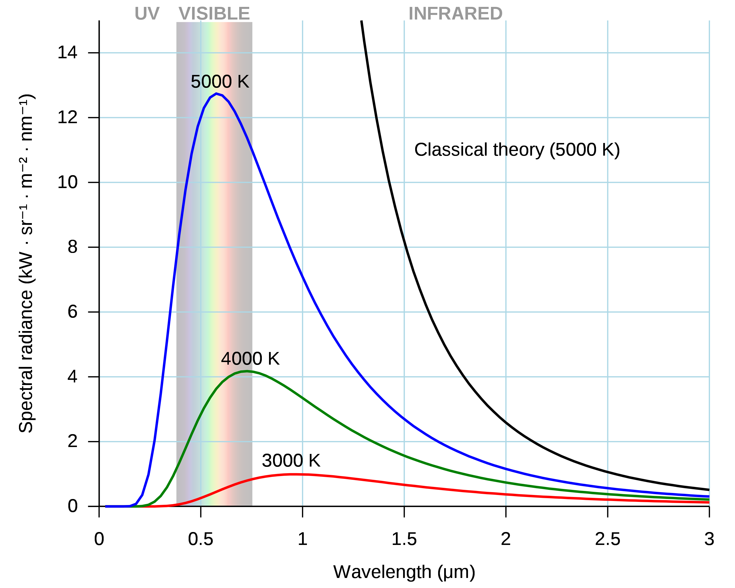

As an object is heated by its environment, the energy it emits spans higher parts of the visible spectrum, apparently shifting in color from dark red to bright white then blue and and potentially even beyond the visible spectrum.

The graph at right illustrates distribution curves for sample color temperatures, which refers to the peak of the distribution of the colors emitted by an object heated to a certain temperatures. These are expressed in Kelvin units, which use the same scale as degrees Celcius but with a zero point offset to absolute zero, so that 0 K is equal to -273.15 °C and 273.15 K is equal to 0 °C. (For each curve, the peak indicates the wavelength with the most photons.)

Objects not hot enough to glow still radiate electromagnetic energy, starting with photons at the end of the spectrum with the longest wavelengths (and thus lowest frequency), which are generally referred to as thermal radiation. If they are hot (energetic) enough, they may emit infrared light, which can be displayed via thermography (thermal imaging), as in thermographic cameras that became practical in the 1970s to provide an early form of artificial night vision.

In 1761, the English scientist, inventor, and lecturer Ebenezer Kinnersley (1711-1778)—a contemporary and correspondent of the American writer, scientist, inventor, statesman, diplomat, printer, publisher, and political philosopher Benjamin Franklin (1706-1790)—demonstrated using the flow of electricity to heat a wire and make it glow with incandescence.

We now call this process Joule heating, through which the amount of electric power flowing through a conductor is limited by its inherent resistance, causing some of the power to be dissipated as heat and increasing the temperature of the conductor. (Please remember the term “power dissipated as heat,” which I wish to promote as an accurate characterization of inefficiency in a circuit and its components.) As the conductor’s temperature increases so does its resistance (in the case of a light bulb, roughly 10 times higher), which further contributes to its incandescence.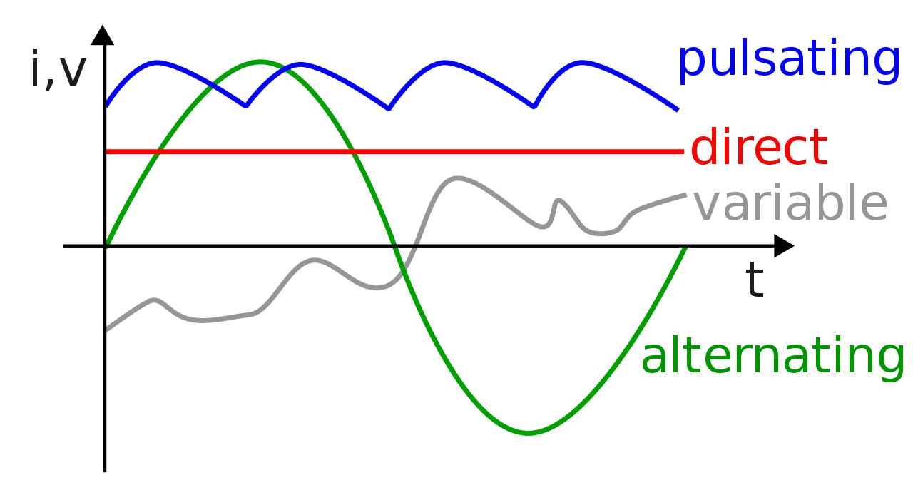

Early experiments with electricity were difficult because sources of electric current were limited. Like the ancient Greeks rubbing amber with fur, early electricity was created using the triboelectric effect (from the Greek prefix tribo- meaning “rub”) starting with electrostatic generators around 1663 rubbing a sulfur ball to convert mechanical power to static electric charge. In 1745, the invention of the Leyden jar allowed small amounts of such a charge to be stored. In 1799, electrochemical cells (and batteries of those cells) were created, starting with the Voltaic pile. The first electromagnetic generators—called dynamos (referring to the charge being dynamic rather than static)—were created in 1831-1866 to convert mechanical force to electrical direct current (DC, formerly called galvanic current). Later, in 1882-1886 alternators (synchronous generators) were made to create alternating current (AC).

Electric Arc Lamps

The first practical electric light was the arc lamp created by Humphry Davy in 1802-1809 and used widely from the 1870s until early in the 20th century. The brightness of this type of lamp made them useful in motion picture studios, but the ultraviolet light they emitted caused eye soreness.

Early arc lamps also had very low efficiencies of only 0.29-1.0%.

Non-Lighting Uses for Ultraviolet Lamps

Arc lamps were replaced for many lighting applications, but remained particularly useful for ultraviolet germicidal irradiation (UVGI) since about 1878, when Arthur Downes and Thomas Blunt published a paper describing the sterilization of bacteria exposed to short-wavelength light. In 1903, Niels Finsen was awarded the third Nobel Prize for Medicine for his use of ultraviolet light against lupus vulgaris (tuberculosis of the skin).

With the rise of the COVID-19 pandemic, in early March 2020, I was tasked with evaluating the practicality of using ultraviolet (UV) light in personal protective equipment (PPE). Because little was yet known about the virus that caused the disease (SARS-CoV-2), I extrapolated using data collected about UV efficacy in deactivating SARS-CoV collected since the 2002-2004 SARS outbreak.

Electric Incandescent Lamps

The incandescent light bulb was developed 1850-1879, with significant improvements 1904-1925 including tungsten filaments replacing carbon filaments, filling them with inert gases, and coating their insides with frosting. (The last may have begun as a fool’s errand, but was successfully invented by Marvin Pipkin, 1889-1977.)

Though improvements continued to be made, the luminous efficacy of incandescent lamps remained less than 5% (about 16 lumens per watt) because most of their output remained below the band of visible light. Incandescent lamps dissipate so much power as heat that in 1963, Kenner Products introduced its toy Easy-Bake Oven, enabing children to bake small cakes using two 100-watt incandescent light bulbs.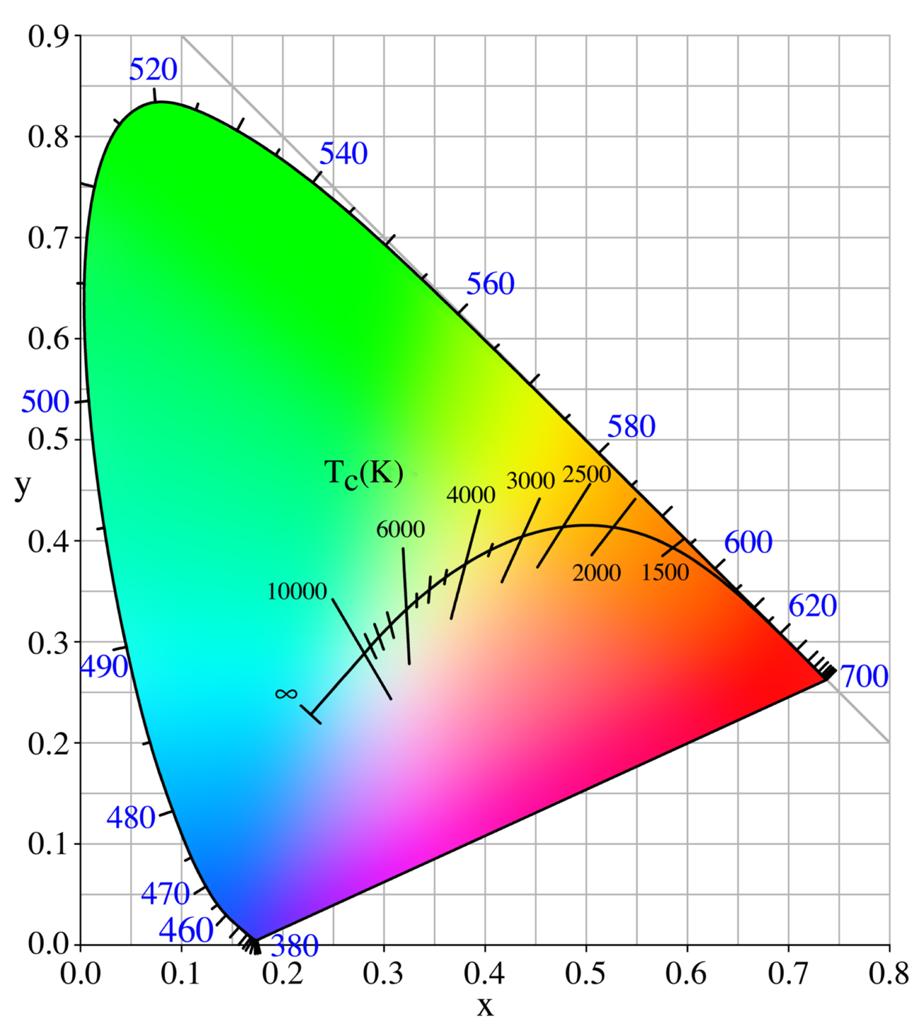

Tungsten filaments are heated by electric current generally to 2000 K to 3300 K. This is limited by tungsten’s melting point, which is 3695 K.

(Note that if power through a circuit is not regulated reasonably, components may change their fundamental state of matter, usually from solid to liquid and—in extreme cases—gas or plasma; when one of the latter has occurred, the component and/or circuit is sometimes described as having released its “magic smoke,” implying—usually with humorous intent—that circuits operate through the passage of smoke through their conductors until it is allowed to leak out. Note also that some electrical engineers and electronic technicians are more successful than others in their attempts at humor.)

For terrestrial photography, the nominal color temperatures used for studio lighting is 3200 K and for sunlight it is 5600 K. (Water vapor in Earth’s atmosphere refracts visible light with shorter wavelengths, giving the daytime sky its blue appearance; beyond the atmosphere—in outer space—the peak color of sunlight is about 3% more blue, with the Sun’s photosphere having an effective temperature of 5772 K.)

Fluorescent Lamps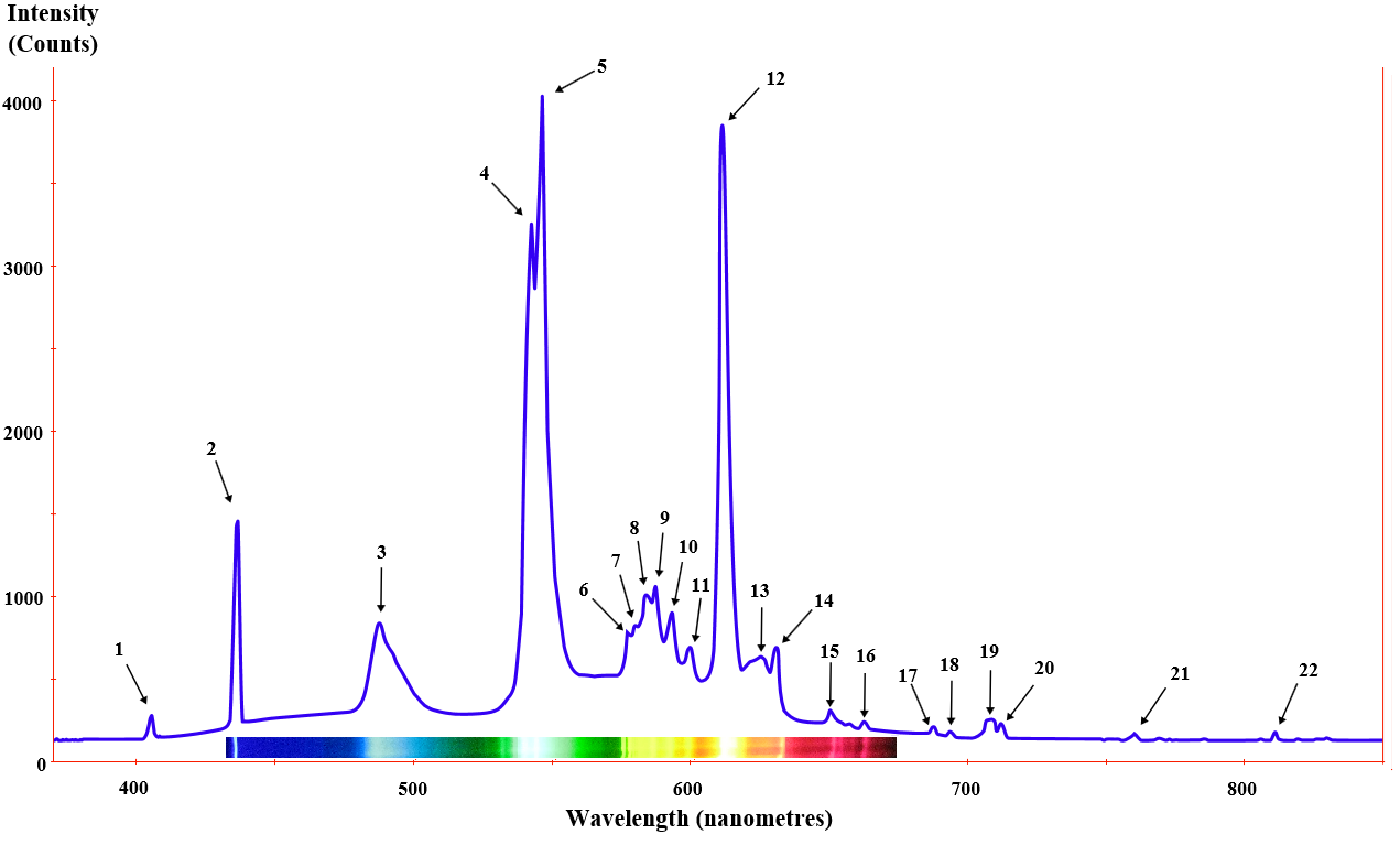

Introduced in 1938, fluorescent lamps are low-pressure mercury-vapor gas-discharge lamps that use fluorescence to produce visible light much more efficiently than incandescent lamps. Fluorescent lamps have a luminous efficacy of 50-100 lumens per watt (about 12% efficient), versus about 16 lumens per watt produced by incandescent lamps (about 1.6% efficient).

By 1951, they produced more light in the United States than incandescent lamps.

Unlike the temperature-dependent normal distribution of colors produced by incandescent lamps, a fluorescent lamp produces light with a complex distribution of colors based on which atomic elements they contain. An example of color distributions from a modern fluorescent lamp is shown in the graph at right, with highest peaks (from left to right) from the excitation of terbium, mercury, and europium, and lower peaks likely also from these and argon.

The spiral compact fluorescent lamp (CFL) was invented in 1976 and they were promoted for their energy efficiency from about 1995 to about 2016. The mercury they contain is highly hazardous (per European Union RoHS directive, California Proposition 65, etc.), so the difficulty of their disposal likely negated any environmental benefit.

Street Lights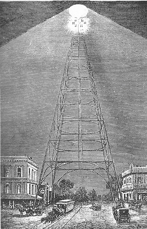

In 1792, the Scottish engineer and inventor William Murdoch (1754-1839) invented gas lighting, and soon thereafter it started being used for street lighting in the United Kingdom. In 1803, the first street lights were installed in the United States.

In 1879, Cleveland, Ohio became the first to demonstrate electric street lighting (on April 29) and San Francisco, California—with two generators from the American engineer and inventor Charles Brush (1849-1929)—became the first city in the nation (and possibly the world) to have a commercial central electric generating station, which incorporated June 30 as the California Electric Light Company—today Pacific Gas and Electric Company (PG&E)—and began service in September.

On March 31, 1880, Wabash, Indiana became the first city to use arc lamps for municipal lighting, turning on four Brush arc lamps mounted on the dome of its city hall.

In San Francisco, electric light was apparently first demonstrated in 1874; after seeing electric light there in 1879, San Jose newspaper publisher J.J. (James Jerome Owen designed a tower similar to the Akron, Ohio moonlight tower built in 1881. The San Jose electric light tower was built that year starting August 11 and dedicated—with six Brush arc lamps (with a total of 24,000 candlepower)—on December 13. The Akron tower collapsed when its supporting cables broke; though the San Jose tower was built with a wider base so no such supporting cables were needed, it collapsed in a storm on December 3, 1915.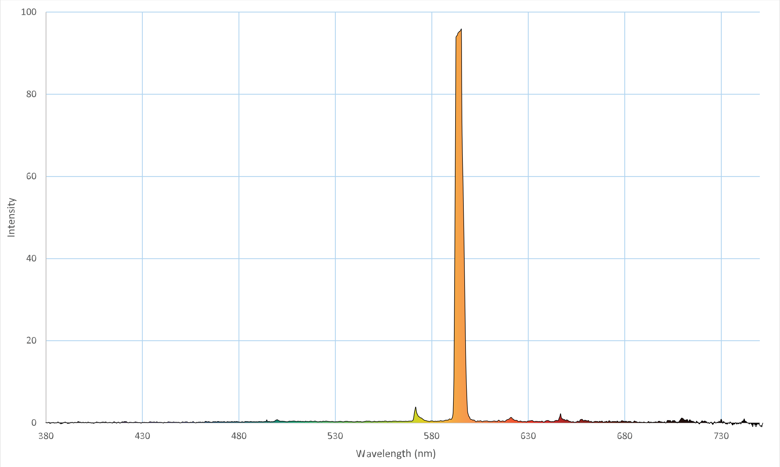

Light pollution caused by street lights often interferes with optical astronomy, including the operation of the nearby Lick Observatory, which is 1283 meters (4209 feet) above mean sea level on Mount Hamilton, east of (and usually visible from) Silicon Valley. (The observatory has operated since 1888 and became part of the University of California system. Its 36-inch refracting telescope was the world’s largest until 1897, and in 1892 it was used to discover the first of the non-Galilean moons of Jupiter.)

To correct this problem, in 1980 the City of San Jose replaced its street lights with low-pressure sodium lamps.

As a type of gas-discharge lamp (specifically a high-intensity discharge lamp, or HID lamp), the band of light emitted is not like the normal distribution of black body radiation seen when heating a solid. Instead, these emit light in a relatively narrow band of the spectrum, as shown at right.

Though my family moved from San Jose to Sunnyvale in 1978, I recall Sunnyvale also changing its street lights around 1980 from what were blue-white—probably mercury-vapor lamps—to the orange low-pressure sodium lamps and more recently to more-efficient LED street lights, which are still easy for the observatory to work around or filter out.

(I also recall playing in snow in the back yard of our San Jose home in 1972 and a somewhat more slushy mess in 1974. Since then, the only snow I’ve seen around here has been at the higher elevations of Mount Hamilton and the ridge of the Santa Cruz Mountains, which is less than 1154 meters or 3786 feet above mean sea level.)

Light-Emitting Diodes

The first commercial light-emitting diodes (LEDs) were introduced by Texas Instruments (TI) in 1962 as an infrared device for signaling via optical fiber. For most applications, LEDs remained prohibitively expensive (about $200 each) until 1968, when Hewlett-Packard (HP) introduced visible red LEDs suitable to replace incandescent lamps and neon lamps used as indicators.

I recall starting to experiment with LEDs around 1979 (indicators, including segmented displays, some in multi-digit matrices), high-brightness LEDs (for roadway signaling) around 2005, and high-power LED lamps (for illumination) around 2010.

The luminous efficiency of LED lamps is about 20%, which is better than that of 12% for fluorescent lamps and about 1.6% for incandescent lamps.

Seeing More Than Stars

Just south of Sunnyvale, California is Cupertino, where I studied at De Anza College (in 1991-1993 and again in 1997-2000, after having moved to Texas and back, and waiting a year to re-establish my residency to qualify for the lower tuition rates for “in-state” residents). There, I had many remarkably good classes, including lighting for film and television, and also astronomy.

At the other school in its district, Foothill College, in early 1996 I had attended a lecture by local astronomer Geoffrey Marcy.

At the Lick Observatory, Marcy had been a pioneer in discovering planets beyond our solar system, also known as exoplanets (extra-solar planets).

Marcy (et al) used an indirect method of detection called Doppler spectroscopy (also known as the radial-velocity method or the wobble method), which had been described in the journal Nature about 3-4 months earlier. In short, the spectrum of light from a distant star can be used to deduce which hot gases produce them (like, for example, the spectrum produced by low-pressure sodium vapor illustrated above); if a planet orbits a star, its mass and proximity will affect the position of the star, and if the orbital plane is aligned closely enough to the direction toward Earth, as as the star moves toward or away from Earth, the Doppler effect will cause the peaks in observed light to shift in the spectrum toward blue or toward red, respectively.

At the time of the lecture, discovery of exoplanets had been confirmed around only three stars (PSR B1257+12 in 1992, 51 Pegasi b in 1995, and 47 Ursae Majoris b in 1996, shortly before the lecture). Before ending the lecture, Marcy presented a potential fourth, which I think was not confirmed. By the start of 2022, confirmed discoveries include 3,629 planetary systems including 4,905 exoplanets.

How We Perceive, Measure, and Describe Light and Color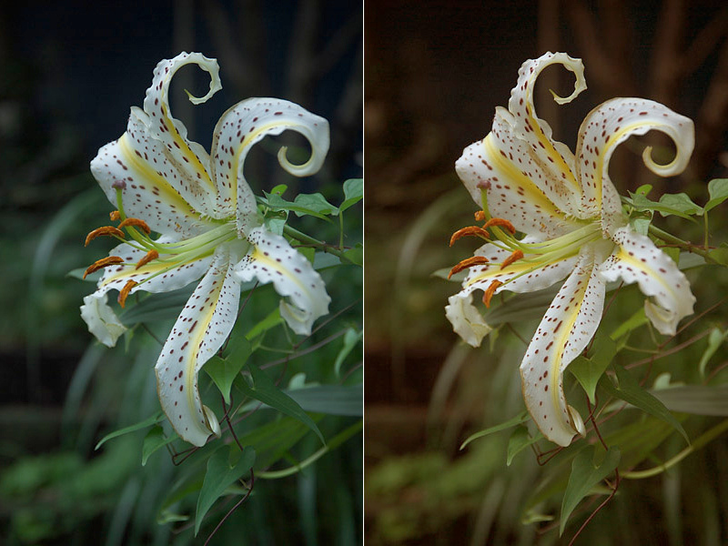

What’s important is that we still perceive something to be the same color whether we look at it in daylight or with artificial light, though light with lower color temperature doesn’t have as many photons at higher frequencies.

When taking photographs or recording motion pictures or video (photography, cinematography, or videography, respectively), we often adjust for the color of ambient light so that when the product is viewed all of its colors will not appear too red nor too blue.

Adjusting the color balance (or white balance) in this way is usually done at the time by selecting a photographic filter or through digital image processing, or afterward through image post processing or video post-processing.

Color Wheels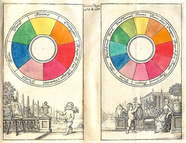

The practice of presenting a circle or wheel with colors organized to illustrate the relationships of neighboring hues appears to have been started by Isaac Newton.

In his 1704 book Opticks, Newton identified seven primary colors and their spectral order: red, orange, yellow, green, blue, indigo, and violet. This sequence may be remembered with the acronym ROYGBIV, especially if pronounced as a person’s name as “Roy G. Biv.”

Newton presented these as colored wedges of a circle. Though Newton put seven colors on his circle (and identified all of them as “primary” colors), many different colors and numbers of colors have been presented on color wheels, as illustrated at right.

Note that in the illustrated seven-color wheel, crimson red (labeled in French as rouge cramoisi) was not one of the colors identified by Newton. It is a composite color, a non-spectral color between red and violet that can be formed only by combining light of at least two different wavelengths. The illustrated 12-color wheel includes this and an additional composite color, purple (pourpre).

Since at least as early as 1762, Newton’s primary colors have been used on spinning discs (a Newton disc) to demonstrate perception of temporal (time-based) color mixing to reproduce white (somewhat imperfectly) from component colors. This is an example of combining light of different colors, or additive color mixing; combining light of enough colors creates light that we perceive as white. This cause of this effect is often described as persistence of vision, which is arguably the foundation for motion pictures (cinema).

Color Models

Many colors are named for where they are found in nature. This works reasonably well, but requires those attempting those giving a description of a color and those attempting to understand it to share a fairly large knowledge of the natural world.

This problem may be solved by creating a color model, which is a method of using a small ordered set of numbers to describe the relationship between a particular color and a small set of widely-known primary colors.

Note that in some color models other terms are used to describe primary colors, such as “primitive” colors in 1725 by Jacob Christoph Le Blon (1667-1741) and in 1830 by J.F.L. Mérimée, (1757-1836); respectively, primary colors and secondary colors were described as “principal hue” and “intermediate hue” in 1905 by Albert H. Munsell (1858-1918), and as “plus color” and “minus color” in 1908 by J. Arthur H. Hatt (lifespan unknown).

Trichromatic Color Models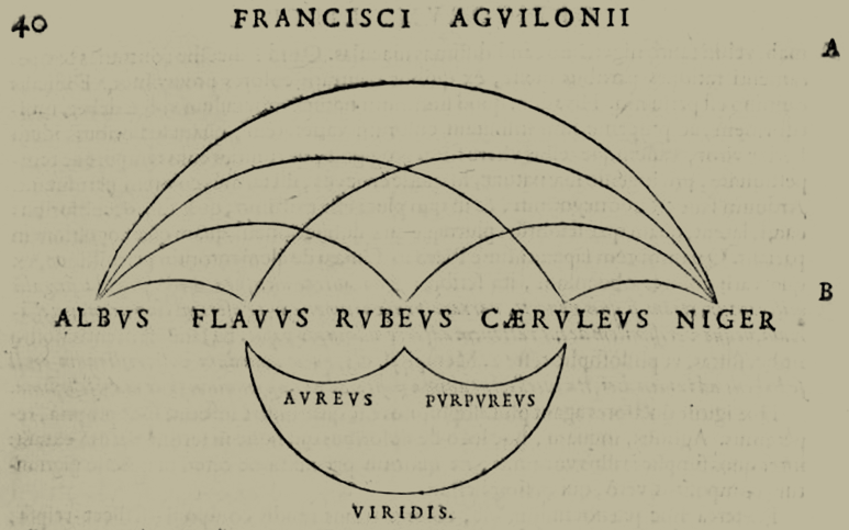

Scholars Scarmiglioni, Savot, and de Boodt (in 1601, 1609, and 1609, respectively) proposed that painters could reproduce any hue by mixing colorants (such as pigments) from only three primary colors. In 1613, the Spanish Netherlands mathematician, physicist, architect, and Jesuit François d’Aguilon (1567-1617, Latinized Franciscus Aguilonius or Francisci Agvilonii) built upon this to illustrate (as shown at right) lines of connection between black (niger) and white (albus), and between both black and white and each of three primary colors: red (rubeus), yellow (flavus), and blue (cæruleus); lines of connection were also drawn for three secondary colors: between red and yellow for orange (aureus), between yellow and blue for green (viridis), and between red and blue for purple (purpureus).

This is an example of combining colorants that absorb light of different colors (the colors that the colorants don’t reflect), or subtractive color mixing; combining enough colorants to absorb all visible light creates a colorant that appears black.

Black and white (nonchromatic, having no color) appear to be included in order to respectively decrease or increase the luminance of a colorant or mixture. Any color could thereby be created by mixing combinations of the five to the desired hue and luminance.

The colors red, yellow, and blue are often abbreviated RYB, and provide the foundation of the RYB color model.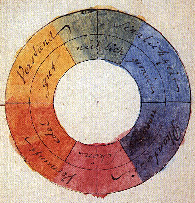

Color wheels with multiples of three colors may be described as having trichromatic (three-color) models. By convention, color models are named after their primary colors, starting with the color of the lowest frequency (usually red) followed by the other two equidistant colors in order of increasing frequency.

For example, the color wheel at right—from Theory of Colours (1810) by the German poet, color theorist, and government minister Johann Wolfgang von Goethe (1749-1832)—includes (clockwise from bottom) red, yellow, and blue (as above).

Similarly, in the previous illustration of two colors wheels, the lowest-frequency color in the 12-color (rightmost) wheel is red. Of the two colors equidistant to red, the color with next-lowest frequency is yellow-green, followed by blue. So, this color wheel could be described as illustrating (counter-clockwise from right) a color model that is red, yellow-green, and violet.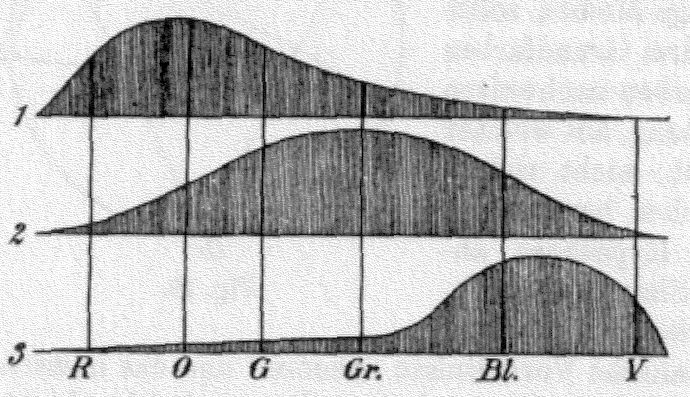

In 1802, the British scientist Thomas Young (1773-1829) postulated the trichromacy of human vision and the existence of three types of color photoreceptor cells (now known as cone cells). In 1852, the German physicist and physician Hermann von Helmholtz (1821-1894) expanded the idea to describe these color photoreceptor cells as being sensitive light of long, medium, and short wavelengths (respectively red orange, green, and violet blue, as illustrated at right), resulting in the Young-Helmholtz theory. (Note the abbreviations of the German words rot, orange, gelb, grün, blau, and violett, meaning red, orange, yellow, green, blue, and violet, respectively.) In 1956, the Swedish-Finnish-Venezuelan physiologist Gunnar Svaetichin (1915-1981) showed that human eyes are most sensitive to yellowish green, cyanish green, and blue.

Though unrelated to trichromacy, it should be noted that in 1892 the German physiologist Ewald Hering (1834-1918) proposed an alternate color theory called opponent process, suggesting that our eyes differentiate three channels: black-versus-white (luminance), red-versus-green, and blue-versus-yellow.

Around 1860, a variation of the RYB color model used red, green, and blue as primary colors to create the RGB color model.

As the RGB color model gained popularity, other color models continued to emerge, such as the one proposed by J. Arthur H. Hatt (published by D. van Nostrand Co.) in 1908 using red, green, and violet as primary colors (which Hatt called “plus” colors, labeling secondary colors “minus” colors). In a 24-color wheel (as illustrated at right), this model includes seven composite colors (the non-spectral colors between red and violet that can be formed only by combining light of at least two different wavelengths) versus only five composite colors needed to fill a 24-color wheel using the RGB model.

Perception-Based Color Models

These models are radiometric, meaning that they describe the absolute power of radiant energy. In contrast, how we perceive light and color are matters for the respective sciences of photometry and colorimetry.

The American painter and art teacher Albert Munsell (1858-1918) created the first perceptually-uniform system to describe colors accurately via numbers by extending the color wheel, adding to the hue angle two additional dimensions for chroma (color intensity, increasing with distance from center) and value (lightness, increasing vertically with height). He described the Munsell Color System in his books A Color Notation (1905, again coincidentally Albert Einstein’s “miracle year”) and Atlas of the Munsell Color System (1915); descriptions published posthumously include A Grammar of Color: Arrangements of Strathmore Papers in a Variety of Printed Color Combinations According to The Munsell Color System (1921) and the Munsell Book of Color (1929).

A Rose, By Any Other Name

My elementary school had two classrooms for each grade level; for what I recall as being a few days when I was 11 years old and in the sixth grade, all of the boys from both classes were corralled into one classroom and all the girls into the other. I and the other boys were taught some unsavory mechanics about biology that many describe as being about “the birds and the bees.”

Since then, I sometimes speculate that the girls learned much more, including the names of many more colors. (How else would they know them?)

The girls seemed to have much larger vocabularies for describing colors (and perhaps many other things).

In contrast, most of us guys could hardly grunt out more than the names of primary colors and secondary colors, sometimes indicating variations with adjectives ending in “-ish” and “-y.” For example, what a girl calls “dandelion,” a boy might only describe as “yellowy orange.” Similarly, boys might use terms such as a “redish blue” or “bluish red” to describe colors along the color wheel to either side of magenta, which boys might call red-blue or blue-red, perhaps depending on their particular political affiliation.

Having grown up in the United States, some of my earliest lessons in color involved drawing crayons.

Since its introduction of Crayola drawing crayons in 1903, the Binney & Smith Company has produced crayons in more than 200 colors, with nearly as many names.

Crayola Color Wheels

Crayola crayons were sold in bulk and, starting in 1905, in assortments of various numbers of colors, including (but not limited to) eight (starting in 1905), 16, 24, 48 (starting in 1949), 52 (produced 1939-1944), 64 (starting in 1958), 96 (starting in 1992), 100 (starting in 2003), and 120 (starting in 1998).

In 1926, Binney & Smith acquired the line of crayons from the Munsell Color Company and its color model based on 10 hues; with it, the Crayola color wheel was born.

As shown in the following table, Munsell Crayola crayons were available in assortments in different sizes, which each included crayons in black, middle gray, and the five “principal hues” at maximum chroma. The next-larger assortment included those and crayons of five the “intermediate hues,” at middle chroma. The largest assortment included all 10 hues, each at both maximum chroma and middle chroma.

Munsell Crayola Crayon Colors (1926-1944)

7 Colors in Assortments of ≥7
black			middle grey
maximum red	maximum yellow	maximum green		maximum blue	maximum purple
5 Additional Colors in Assortments of ≥12
middle red purple	middle yellow red	middle green yellow		middle blue green	middle blue purple
10 Additional Colors in Assortments of 22
maximum red purple	maximum yellow red	maximum green yellow		maximum blue green	maximum blue purple
middle red	middle yellow	middle green		middle blue	middle purple

Key:
“principal hue”
“intermediate hue”

Changes to the Crayola color wheel included the following.

1930

Expanded to 12 colors, adding orange as a principal hue and dividing the intermediate hue red-yellow into red-orange and orange-yellow

1935

Blue revised (made darker)

1949

Violet revised

1958

Violet revised and relabeled as “violet (purple);” six intermediate hues added (12 intermediate hues, 18 total in color wheel)

1990

Four intermediate hues removed (leaving 8 intermediate hues, 14 total in color wheel)

The following table includes the names of the colors (as labeled on the crayon wrappers) included in assortments of up to 64 colored crayons. Shown below some colors are the colors they replaced.

Note that in 1930-1935 the 16-color assortment included “neutral grey” (sic) in place of “rose pink,” and a 52-color assortment was produced 1939-1944. (Read more about the history of Crayola crayons.)

Crayola Drawing Crayon Colors

8 Colors in Assortments of ≥8 (≥1905)
black (≥1903)	brown (Van Dyke brown 1903-1935)	red * (≥1903)	orange * (≥1903)	yellow * (≥1903)	green * (≥1903)	blue * (≥1958)	“violet (purple)” * (≥1958, 1930-1949)
						blue (1935-1949; medium blue 1949-1958)	violet (1903-1930)
						blue (1903-1935; celestial blue 1935-1949; azure blue 1949-1958)
8 Additional Colors in Assortments of ≥16 (≥1930)
white (≥1903)	carnation pink (pink 1903-1917; rose pink 1903-1958)	red orange * (≥1930)	yellow orange (≥1930)	yellow green * (≥1930)	blue green (maximum blue 1926-1949; middle blue green 1949-1958)	blue violet (violet 1949-1958)	red violet * (≥1930)
8 Additional Colors in Assortments of ≥24
gray (middle grey 1926-1930; neutral grey 1930-1956)	scarlet * (torch red <1998)	apricot (≥1958)	bluetiful (≥2017)	green yellow * (≥1958)	cerulean * (≥1990)	indigo (≥1999)	violet red (≥1958)
		orange red * (1958-1990)	dandelion (1990-2017)		green blue * (1958-1990)	thistle * (1958-1999; light magenta 1949-1958)
			orange yellow * (1958-1990)		cerulean blue (1949-1958)	violet blue * (1958-1990; blue violet 1930-1958)
8 Additional Colors in Assortments of ≥32
timberwolf (≥1993)	chestnut (Indian red 1903-1999)	melon * (≥1958)	peach * (flesh tint 1903-1949; flesh 1949-1956; pink beige 1956-1958)	tan * (≥1958)	sky blue * (≥1949)	cadet blue (≥1958)	wisteria (≥1993)
16 Additional Colors in Assortments of ≥48 (≥1949)
salmon (≥1949)	sepia (≥1958; 1935-1944)	mahogany (≥1949)	macaroni and cheese (≥1993)	goldenrod (medium chrome yellow 1903-1910; medium yellow 1910-1958)	olive green (≥1903)	cornflower * (≥1958)	purple mountain majesty (≥1993)
mauvelous (≥1993)	tumbleweed (≥1993)	raw sienna (≥1958)	burnt sienna (≥1903)	spring green * (≥1958)	granny smith apple (≥1993)	sea green * (light green 1949-1958)	lavender (≥1958)
		raw sienna (1903-~1910)					lavender (1949-1958)
16 Additional Colors in Assortments of ≥64 (≥1958)
silver * (metallic; ≥1903)	brick red (≥1958)	bittersweet (≥1958)	burnt orange (≥1958)	asparagus (≥1993)	robin’s egg blue (≥1993)	pacific blue (≥1993)	plum (≥1958)
gold * (metallic; ≥1953)	magenta (permanent magenta 1903-1914)	tickle me pink (≥1993)	wild strawberry (≥1990)	forest green * (dark green 1949-1958)	turquoise blue (≥1958)	periwinkle * (≥1958)	orchid * (medium red violet 1949-1958)
gold * (metallic; 1903-1944)	brilliant rose (1949-1958)				light blue (1958)

Key:
“principal hue” on Crayola color wheel (six from 1930 to present)
“intermediate hue” on Crayola color wheel (six from 1930 to 1958, 12 from 1958 to 1990, eight from 1990 to present)
Italic names are unique to Crayola
* indicates a Crayola color that differs from others of the same name

Color Codes

Colors used to encode information form a color code. Though these might vary by the contexts in which they are used, some code sequences of numbers as sequences of colors following their order in the visible spectrum.

General Electronic/Resistor Color Code

A sequence similar to Newton’s primary colors, the electronic color code has been used to encode the nominal values (and sometimes part numbers) of components of electronic circuits starting with axial-lead resistors in the 1920s.

As shown in the following table, the sequence of the electronic color code starts with black and brown followed by Newton’s primary colors—the “Roy G. Biv” acronym ROYGBIV—minus indigo (all of which have been Crayola colors since 1903), and ending with gray (a 1926 Munsell Crayola color) and white (another 1903 Crayola color).

Electronic Color Code

Number	Color	Abbr.	Name
0		BLK	black
1		BRN	brown
2		RED	red
3		ORA	orange
4		YEL	yellow
5		GRN	green
6		BLU	blue
7		VIO	violet
8		GRY	gray
9		WHT	white

On axial components, colored bands could easily be read backward, yielding an incorrect value (or part number). Correct values (other than valid part numbers) follow the E series of preferred numbers, which is based on a system of preferred numbers called a Renard series (or sometimes Renard numbers), created by French military engineer Charles Renard (1847-1905), which was adopted by the International Organization for Standardization (ISO) in the 1950s as the international standard ISO 3; in 1952, the International Electrotechnical Commission standardized the E series as IEC 63.

These colors are also used widely on individual wires and on wires within cables. In many contexts they follow the order above.

Thermostat Control Color Code

Electric thermostats control heating, ventilation, and air conditioning (HVAC) in residential and commercial buildings control generally equipment via cables with wires color-coded to provide the following functions. Generally, the operate using 24 VAC (volts alternating current) with two to five wires, though 24-volt thermostats could use more wires to control functions of complex systems.

The table below includes the most common wire functions used with 24 VAC thermostats.

Thermostat Control Wire Colors

Code	Color	Name	Function	Memory Aid
R		Red	24 VAC return for signals*	Return = red
W		White	Signal to run heat (when connected to 24 VAC above)	With white snow we run the heat.
Y		Yellow	Signal to run cooling (when connected to 24 VAC above)	With yellow sun we run the cooling.
G		Green	Signal to run fan (when connected to 24 VAC above)**	With green spring leaves we run the fan.
C		Blue	24 VAC common supply (used to power clocks, memory, etc.)	Common = cobalt blue

* Note that some systems may also include red wires labeled Rh and Rc, which are 24 VAC isolated returns for heat and cooling, respectively. These are often connected together, and connected to R if present.

** In forced-air systems, running the fan is implied when the heat signal or cooling signal is active. Asserting the fan signal without either of these should run the fan only.

Telephony Color Code

Noteably different is the color code used by in the United States by Bell System telephone operators starting in the 1950s, which renames gray as slate and follows its own 25-pair color code. This splits the 10 colors above into five major colors and five minor colors. Respectively, these are used to make the tip and ring connections historically found on a phone plug. The orders of the major and minor colors are shown in the table below, and may be remembered with mnemonic devices for the first letter of each color, such as “When running backwards you’ll vomit” and “Bell operators give better service,” respectively. The wires in newer cables generally include a second color added as a stripe along their length, or sometimes as bands spaced evenly across them; for paired conductors, the second color is the first color of the paired conductor.

Bell System 25-Pair Wire Insulator Color Code (RJ21)

Group	Pair	Ring (Minor Color)			Tip (Major Color)
		Pin	Color/Stripe		Pin	Color/Stripe
1	1	1	—	blue/white	26	—	white/blue
1	2	2	—	orange/white	27	—	white/orange
1	3	3	—	green/white	28	—	white/green
1	4	4	—	brown/white	29	—	white/brown
1	5	5	—	slate/white	30	—	white/slate
2	1	6	—	blue/red	31	—	red/blue
2	2	7	—	orange/red	32	—	red/orange
2	3	8	—	green/red	33	—	red/green
2	4	9	—	brown/red	34	—	red/brown
2	5	10	—	slate/red	35	—	red/slate
3	1	11	—	blue/black	36	—	black/blue
3	2	12	—	orange/black	37	—	black/orange
3	3	13	—	green/black	38	—	black/green
3	4	14	—	brown/black	39	—	black/brown
3	5	15	—	slate/black	40	—	black/slate
4	1	16	—	blue/yellow	41	—	yellow/blue
4	2	17	—	orange/yellow	42	—	yellow/orange
4	3	18	—	green/yellow	43	—	yellow/green
4	4	19	—	brown/yellow	44	—	yellow/brown
4	5	20	—	slate/yellow	45	—	yellow/slate
5	1	21	—	blue/violet	46	—	violet/blue
5	2	22	—	orange/violet	47	—	violet/orange
5	3	23	—	green/violet	48	—	violet/green
5	4	24	—	brown/violet	49	—	violet/brown
5	5	25	—	slate/violet	50	—	violet/slate

(My friend and neighbor across the street since 1978, Steve Peters had a notable career working for AT&T from 1957 to 1987. I recall that around 1990, the AT&T research facility in north Sunnyvale where he likely had worked and a few other other buildings—including where I had seen programmable logic pioneer Monolithic Memories Incorporated—were demolished to build the AMD headquarters campus.)

Other Color-Coded Wire and Cable

Other (non-telephone) wire and cable follows the color code in spectral order shown earlier. However, because natural numbers are used to count conductors, the sequence starts with brown and black is used to indicate the tenth conductor.

For example, ribbon cables (invented in 1956) are available with color-coded insulation over their conductors (“rainbow” cable), the color sequence starting with brown and repeating every 10 conductors. On ribbon cable that is otherwise monochromatic (such as gray, which is common), the intended orientation of the cable is indicated by coloring only the first conductor (often red).

In addition to indicating which position a wire occupies within a cable (or within a bundle inside a large cable), the color of a wire’s insulator can also suggest its function within the context of the system it is used in.

AC Power Wire Colors

For example, electrical wiring in North America for high-voltage alternating current (i.e. line power or mains power) follow national regulations; in the United States, the National Electrical Code (NEC) specifies which colors of insulation (or other marking) may be used on wires used to make certain connections, as shown in the following table. (Note that of the colors in the previous, the use of violet is not specified.)

Wire Insulator Colors for Power in North America

Function	Color
	120, 208, or 240 VAC		277 or 480 VAC
Earth ground	X	bare (non-insulated)
		green
	—	green with a yellow stripe (isolated systems)
Neutral return	X	metallic silver
		white	—	gray
Power phases	X	metallic brass
		black for first phase		brown
		red for second phase		orange (also high-leg delta)
		blue		yellow

Automotive Wire Colors

In many other contexts, color codes are not regulated but are adopted by convention.

One example is automotive audio, as shown in the following table.

Common Wire Insulator Colors for Automobile Audio

Color		Function
	black	0V return (chassis/“ground”)
	red	+12V power, switched (running/accessory)
	orange	dash lights/dimmer
—	orange with black stripe	remote power amplifier ground/return
	yellow	+12V power, non-switched (battery/standby)
	green	speaker, left rear +
—	green with black stripe	speaker, left rear −
	blue	antenna amplifier/power antenna “on” signal
—	blue with white stripe	remote power amplifier “on” signal
	violet	speaker, right rear +
—	violet with black stripe	speaker, right rear −
	gray	speaker, right front +
—	gray with black stripe	speaker, right front −
	white	speaker, left front +
—	white with black stripe	speaker, left front −

PC Power Supply Wire Colors

Another example is the set of colors used to connect direct current (and related signals) on power supply units (PSUs) derived from the 1981 IBM Personal Computer (PC) including the 1983 IBM Personal Computer XT (PC/XT), the 1984 IBM Personal Computer AT (PC/AT), and the 1995 Intel ATX (Advanced Technology eXtended) specification, as shown in the following table.

Common Wire Insulator Colors for PC/ATX Power

Color		Function
—	black	0V return (chassis/“ground”)
	brown	+3.3V sense (feedback to power supply)
	red	+5V (also for HDD/SSD/SATA)
	orange	+3.3V (also for SATA)
	yellow	+12V (also for RS-232, HDD/SSD/SATA, CPU VRM)
	green	power supply enable (to power supply)
	blue	−12V (for RS-232)
	violet	+5V standby (for RTC, wake-on-LAN)
	gray	“power good” (PG) signal (from power supply)
	white	−5V (AT, phased out in ATX)

In 2001, I was tasked with designing the power supply and regulation subsystem for the first computer with the x86-64 microprocessor architecture still used by most personal computers and servers today. At the time, I was designing what would become the Newisys 2100, intended to be the first (and smallest) in a series of computers with two, four, and eight units of the first 64-bit AMD microprocessor, code-named K8 Hammer (or SledgeHammer) and marketed as Opteron.

Several things made this project interesting to me.

• I got to design a significant part of a new computer around a new microprocessor with an architecture intended to compete with head-on with Intel’s IA-64 (which seemed like a big gamble at the time), and I got work with some really bright engineers both at Newisys and at AMD across town (going from southwest Austin to AMD in the southeast), who had internally code-named our project “Beachhead.”
• Anticipating scaling the design was tricky, as was squeezing the two-processor design into 19-inch rack with one-unit (1U) height (nominally 1.75 inches or 44.45 millimeters).
• As with prior computers, it was economical to use a voltage regulator module (VRM) for each microprocessor; because the microprocessor was so new that no VRMs for it existed yet, I found Artesyn Technologies (which I believe was part of Emerson Electric at the time) and outsourced that part of the design to it.
• To optimize performance, the computers needed to provide Operating System-directed configuration and Power Management (OSPM, part of the 1996 standard Advanced Configuration and Power Interface, or ACPI) with the ability to vary its regulated voltages (nearly all of them) from nominal to margins of about ±10%, controlled by the software running on them, in this case via a service processor (“management blade”) built on the PowerPC architecture created by the AIM alliance (Apple-IBM-Motorola) co-founded in 1991 by my second-line manager Phil Hester, who later became AMD’s chief technology officer (CTO); the System Management Bus (SMBus) standard had only existed since 1994 and its variant Power Management Bus (PMBus) wasn't created until 2004, and I found that the most economical way to achieve the goal (at the time) was to design (and document for the software team) a simple parallel interface (four to eight bits wide) to registers controlling resistor-ladder DACs (digital-to-analog converters) and a single complex programmable logic device (CPLD) to vary the five-bit core voltage identification (VID) code from two microprocessors to their VRMs.
• Allowing this much variance on so many regulators meant that my power budget needed to include wide ranges.
• For the bulk power supply unit (PSU), I had found Transistor Devices Inc. (TDI), a well-qualified vendor that satisfied me with a reasonable bid within our budget; after some growing pains caused me to leave Newisys, the first person to replace me reportedly replaced the TDI PSU with one from a less-reliable vendor, causing some units to catch fire in the field. (About two years after I left, on another project I corrected the work of another one of my “replacements” who had rather foolishly neglected to make the common return connection required on an RS-232 interface, causing it to function only when connected to certain computers.)

USB Wire Colors

A technological descendant of the 1979 Atari SIO (serial input/output) bus, the USB (Universal Serial Bus) standard introduced in 1996 combines conductors for power supply and return and a differentially-signalled twisted pair for bi-directional serial data. Common colors used are in the following table.

Wire Insulator Colors for USB

Pin	Color		Function
1		red	+5V power supply
2		white	D− (negative data)
3		green	D+ (positive data)
4	—	black	0V power return (“ground”)

Television

Although electronic television systems were invented in the United States in the 1920s, they were first produced in 1934, incompatible until standardized in 1941, and entered mass production in 1946. They displayed images using only various intensities of gray, commonly called “black and white” though better described as monochromatic.

Each television set (receiver set) had a cathode-ray tube (CRT), which would draw a picture by causing the phosphor inside its front surface to glow through a type of photoluminescence called phosphorescence, specifically cathodoluminescence caused by an electron beam. In raster-based CRTs (versus vector displays), the beam scans one line at a time from left to right, top to bottom, then starts at the top again drawing the lines between the first (interlacing two fields to form one complete frame. Several levels of brightness or luminance could be created by coding the beam with an analog signal.

Starting in 1954, RCA began producing CRTs for color televisions by interweaving phosphors of the colors red, green, and blue (RGB), each separated by a shadow mask. (In 1968, Sony introduced its Trinitron CRTs, which used each use an aperture grille instead.)

Doing this divided the drawing surface of the CRTs into discrete “picture elements,” usually now known by the portmanteau pixels. (This might sometimes be shortened further to “pel,” though I’ve only found that term used while working for IBM in 1988 to describe the “megapel” displays on its RT PC workstations; with the 4:3 aspect ratio being common at the time, these displays would have had a resolution of at least 1155 pixels wide and 866 pixels high.)

Computer Displays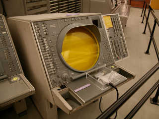

Possibly the earliest example of a computer with a CRT display (at least in the United States) were the 24 digital computers (each built from walls of vacuum tubes and weighing about 250 tons) developed in the 1950s by MIT and built by IBM for the United States military Semi-Automatic Ground Environment (SAGE) system. These were designated AN/FSQ-7 Combat Direction Central—from “Army-Navy/Fixed Special eQuipment”—and sometimes shortened “Q7.” As shown at right, its operator consoles included a large round vector display and a light gun that would be pressed against the display to activate a switch, operating more like a light pen. (Further reflecting when the console was created, it also included a cigarette lighter and an ash tray.)

Monochrome CRT displays were added to commercially-available general-purpose computers starting with the 1959 Digital Equipment Corporation (DEC) PDP-1 minicomputer and the 1964 Control Data Corporation (CDC) 6600, which had an operator console with two large round vector displays and is generally considered to be the first successful supercomputer. (For about the first 10 years of my life, my father worked for CDC; he described a program that would draw and slowly animate eyes on the console’s two displays.)

In 1962, a game was created that could be played on the PDP-1 called Spacewar!. This inspired the first coin-operated video game (a special-purpose computer), Computer Space, which was released in 1971 but—apparently due to its complexity—not a commercial success. In 1972, Magnavox released its home video game Odyssey. Later that year, the developers of Computer Space formed Atari and created the first commercially-successful coin-operated video game, Pong. Home versions followed starting in 1975, as did coin-operated variants Breakout in 1976 and Super Breakout in 1978. The latter two continued to use less-expensive monochrome CRTs but with overlays to produce their distinctive color bands.

The first commercial general-purpose computers with color CRTs were probably the 1975 DEC VT52 terminal and the 1977 Apple II microcomputer. (The latter was part of the “1977 trinity” of three microcomputers released that year, the other two being the monochrome Commodore PET 2001 and Tandy Radio Shack TRS-80.)

Note that Apple later introduced black-and-white models (Lisa and Macintosh in 1983 and 1984, respectively) using a microprocessor made by Motorola; its name is a portmaneau of motorcar and Victrola (branded in 1906), which was named after granola (1886), pianola (1901), and—perhaps with some irony—Crayola (1903). (As mentioned earlier, monochrome CRTs had higher resolution because they did not interleave multiple colors of phosphor on the same surface.)

Early portable computers had CRTs, causing their size and weight to resemble luggage (and earning the description “luggable”); examples include the Osborne 1 (1981), Kaypro II (1982), and Commodore SX-64 (1984). These were replaced by laptop computers with flat-panel displays such as the IBM PC Convertible (1986) and Apple Macintosh Portable (1989).

Flat panel displays replaced CRTs on desktop computers about 20 years later.

Computer Color Spaces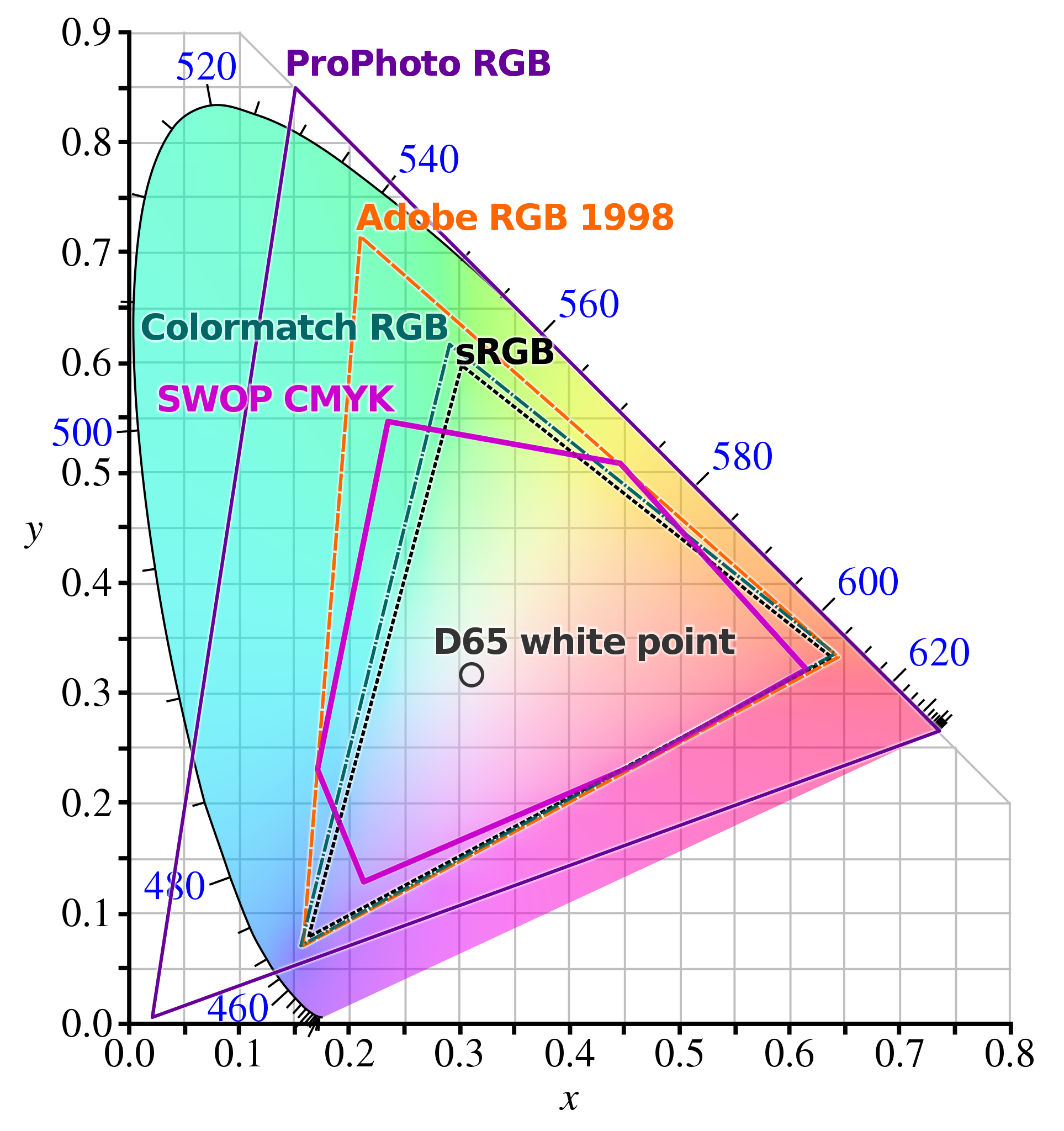

A color space defines a gamut, which is a complete subset of colors that can be reproduced.

The darkest and lightest limits of a display device are its black level and white level, respectively. Those two levels and levels between them form the device’s dynamic range.

A display device’s dynamic range may be represented numerically, for example as 0% (darkest black) to 100% (lightest white).

Digital computers represent integer values as binary (base 2) numbers with “binary information digits” or bits, which may each be off or on, represented numerically as zero or one (0 or 1), respectively; these were named in 1947 by John Tukey (1915-2000).

Binary is also the least efficient positional numeral system, so groups of three or four bits are often represented using octal (base 8, used widely by Digital Equipment Corporation) or hexadecimal (base 16) digits, respectively. Each octal digit represents binary numbers in the range 000 through 111, and each hexadecimal digit represents binary numbers in the range 0000 through 1111, using the letters A through F to represent values 10 through 15. (Letters may be used in either majuscule or minuscule—upper case or lower case—but generally should be used consistently.) By convention, hexadecimal numbers are often differentiated from decimal (or numbers having other bases) with prefixes such as “0x” or the pound sign (“#”), or the suffix “h“.

Each pair of hexadecimal digits represents eight bits, which is called a byte. A byte can represent one of 256 values, usually representing the decimal range 0 through 255, which in hexadecimal is #00 through #FF.

Today, color values are commonly represented as a hexadecimal triplet (three bytes of eight bits each, totalling 24 bits) containing one byte for each of the primary colors red, green, and blue (RGB), in that order. (Although systems representing color with more than 24 bits have been created, their smaller differences in colors are generally imperceptible.)

To represent colors uniformly across computer systems and devices, in 1996 several companies created a color space defining a common “standard RGB,” usually abbreviated sRGB.

The displays of earlier computers were limited by the high cost of memory at the time.

The number of bits required to represent each pixel in color systems is called color depth. Including monochome systems, a more-general term is bit depth. (Note that this differs from Z order, which refers to the order in which drawn objects may be stacked so that only the topmost object is drawn.)

To minimize the amount of memory needed, some early computers used indexed color modes, which—like in paint-by-number sets—assigned a small color number for each pixel that would select a color from the subset of colors that could be displayed (the gamut); this subset is called a palette or color look-up table (CLUT). (Atari 8-bit computers could also display more colors on the screen simultaneously—though not on the same line—by performing display list interrupts.)

The bit depths of various display technologies are shown in the following table.

Per-Pixel Bit Depths of Various Systems

Bits	Levels/Colors	Example
1	2-level monochrome (black & white)	Apple Lisa (1983) Apple Macintosh (1984)
1	2 of 128 colors (indexed 7 bits)	Atari 800 modes 4, 6 (1979)
1	4 colors (via CRT color artifacts)	Atari 800 mode 8 (1979)
2	4-level monochrome (grayscale)	IBM Monochrome Display Adapter (1981)
2	4 colors (via CRT color artifacts)	Apple II Hi-Res (2 artifact color modes, 1977)
2	4 of 128 colors (indexed 7 bits)	Atari 800 modes 3, 5, 7 (1979)
4	16 colors (direct* RGBI)	Apple II Low-Res (1977) IBM PC CGA (1981)
4	16 of 16,777,216 colors (indexed 8-8-8 RGB)	Apple Macintosh II 4-bit version (1987)
6	64 colors (direct 2-2-2 RGB)	IBM PC EGA (1984)
8	256 colors (direct 3-3-2 RGB)	IBM PS/2 VGA Mode 13h (1987)
8	256 of 262,144 colors (indexed 6-6-6 RGB)	IBM PS/2 VGA (1987)
8	256 of 16,777,216 colors (indexed 8-8-8 RGB)	Apple Macintosh II 8-bit version (1987)
15	32,768 colors (direct 5-5-5 RGB)	Super VGA (1988)
16	65,536 colors (direct 5-6-5 RGB)	Super VGA "high color"
18	262,144 colors (direct 6-6-6 RGB)	Super VGA
24	16,777,216 colors (direct 8-8-8 RGB)	Super VGA "true color" (circa 1992)

*: RGBI uses one bit for each red, green, blue, and intensity; CGA and similar systems substitute brown for dark yellow (a color exception to the otherwise-normal color index)

In the following tables, the component hexadecimal values in each RGB triplet have been normalized to represent { 0%, 25%, 50%, 75%, 100% } as { 00, 3F, 7F, BF, FF }.

Note that four-bit RGBI (red, green, blue, and intensity) has only four values that are nonchromatic, at which red, green, and blue are at the same levels; these are { 0000, 0001, 1110, 1111 }. So, RGBI represents intensities of { 0, 1/3, 2/3, 1 } as black, two gray levels, and white, as included in the following table.

Sample Luminance Levels

Name & Year Named		Level	24-Bit Value	Light- ness
black	<1500		#000000	0%
dark gray (non-RGBI)			#3F3F3F	25%
dark gray (RGBI)			#555555	33%
gray	700		#7F7F7F	50%
light gray (RGBI)			#AAAAAA	67%
silver	1481		#BFBFBF	75%
white	<1150		#FFFFFF	100%

In the 1970s, methods of describing colors similar to Munsell’s were introduced for computers, including the color models HSL and HSV, respectively hue, saturation, and luminance and hue, saturation, and value. The latter is also known as HSB, for hue, saturation, and brightness; note that terms value and brightness are used interchangeably. Though these are used less commonly than RGB, examples of value, brightness, and lightness are also included in the following table.

For simplicity, the color table below includes only regular intervals between hue angles and maximum (100%) saturation and value. Note that colors in the color wheel between violet and red (respectively the highest and lowest frequencies of visible light) are composite colors, which can be created only by mixing light with red and blue component colors.

As described earlier, the frequency at which a photon oscillates depends upon the speed at which the photon travels and the oscillation’s wavelength. This relationship is conventionally described by the equation

ν = c ÷ λ

in which:

ν (nu)

is the photon’s frequency in hertz (Hz) & often on the order of terahertz (1 THz = 10¹² Hz),

λ (lambda)

is the photon’s wavelength in meters (m) & often on the order of nanometers (1 nm = 10^-9 m), and

c

is the speed of light (the photon’s speed), which (as described earlier) in a vacuum is 299,792,458 m/s.

Additionally, a photon’s energy can be expressed as follows:

E = h · ν = (h · c) ÷ λ

in which:

E

is a photon’s energy in electronvolts (eV),

h

is the Planck constant, which is about 4.135667696×10⁻¹⁵ electronvolts per hertz (eV/Hz), and

ν (nu)

is the photon’s frequency in hertz (Hz) & often on the order of terahertz (1 THz = 10¹² Hz)

Colors of RGB 24-Hue Wheels at 100% and 50% Brightness

Color Wheel					100% Value/Brightness					50% V/B			Physical Properties
Hue Angle	Set				Name & Year Named		Color	24-Bit Value	Light- ness	Name & Year Named		Color	λ (nm)	ν (THz)	E (eV)
0°	Primary				red			#FF0000	50%	maroon	1789		620-770	400-484	1.16-2.00
15°				Qua	vermilion	1289		#FF3F00	42%
30°			Ter		orange	1502		#FF7F00	50%	brown	1000		590-620	484-508	2.00-2.10
45°				Qua	amber	1500		#FFBF00	50%
60°		Sec			yellow	700		#FFFF00	50%	olive	<1500		570-590	508-526	2.10-2.18
75°				Qua	lime	1890		#BFFF00	50%				564	532	2.28
90°			Ter		chartreuse	>1764		#7FFF00	50%
105°				Qua	harlequin	1923		#3FFF00	50%
120°	Primary				green *	~700		#00FF00	50%	green *	~700		495-570	526-606	2.18-2.51
135°				Qua	erin	≤1842		#00FF3F	50%
150°			Ter		spring green	1766		#00FF7F	50%				505	594	2.46
165°				Qua	aquamarine	1598		#00FFBF	75%
180°		Sec			cyan **	1879		#00FFFF	50%	teal	1917		490-520	575-610	2.38-2.53
195°				Qua	capri	1920		#00BFFF	50%
210°			Ter		azure	1374		#007FFF	50%
225°				Qua	cerulean	1590		#003FFF	33%
240°	Primary				blue			#0000FF	50%	navy	1813		450-495	606-668	2.51-2.76
255°				Qua	indigo	1289		#3F00FF	42%				420-450	668-690	2.76-2.95
270°			Ter		violet	1672		#7F00FF	50%				380-420	690-790	2.95-3.26
285°				Qua	purple †	<1000		#BF00FF	58%				These colors are formed only by mixing red and blue components.
300°		Sec			magenta ††	1859		#FF00FF	67%	purple †	<1000
315°				Qua	cerise †	1845		#FF00BF	58%
330°			Ter		rose ‡	1382		#FF007F	50%
345°				Qua	crimson †	1400		#FF003F	42%
360°	See 0°

Key:

*

At 100% brightness, the X11 name is green and W3C name is lime; at 50%, the W3C name is green.

**

Cyan is sometimes called aqua; with a hex value of #0FFFFF, aqua is 6.25% brighter.

†

Approximate values:

• Purple may be represented like magenta at half its brightness as RGB #7F007F (HSV 300°, 100%, 50%)
• Cerise may be represented as RGB #DE3163 (HSV 343°, 78%, 87%)
• Crimson may be represented as RGB #DC143C (HSV 348°, 91%, 86%)

††

Magenta is the X11 name, fuchia is the W3C name

‡

Rose is sometimes identified as either of the “web-safe” colors #FF00CC (closer to magenta than to red, with a hue angle near 320 degrees) or #FF0077 (closer to red than magenta, with a hue angle of about 340 degrees).

In Memoriam

I began writing this page shortly before the 2021 death of my childhood mentor and lifelong friend LaFarr Stuart, who in the early 1960s pioneered playing music on computers (made with vacuum tubes at the time) and in the early 1980s co-founded and retired from a maker of logic semiconductors as he introduced me to electronics and computers.